Can hidden memory be rewritten using one observable time?

One observable time can carry a larger predictive state

An observable equation with memory may depend on its past because the displayed state omits information retained elsewhere. Restoring that information can turn the evolution into a first-order system using one time parameter. This does not make memory unreal; it identifies where the predictive information resides.

For DTT, inner generation and outer completion name distinct operational roles. The six inner levels are nested dependencies, not a requirement for six independent laboratory time variables. A mathematical rewriting with one clock does not by itself disprove those roles. It does, however, show that a memory kernel alone cannot establish a unique temporal ontology.

The productive question is what the source framework restricts: the dimension and physical cost of retained memory, the allowed interventions, the shape of the kernel or its relation to clocks and geometry. The predictive-record programme provides a precise starting point.

Derive the memory term instead of inserting it

Take finite vectors x,z and constant matrices with equations ẋ=Ax+Bz and ż=Cx+Dz. Solving the second equation yields z(t)=e^tDz(0)+∫₀ᵗe^(t−s)DCx(s)ds. Substitution gives

The initial-memory term is part of the prediction. Setting it to zero is a preparation assumption, not an algebraic simplification valid for every source state. An applied control can be included in the first-order system, but its coupling to the hidden variables must also be carried through the elimination.

Conversely, a memory equation with this kernel has the displayed auxiliary-state realization. The two forms give the same visible trajectories when their initial data and controls are matched. They can differ only if one formulation is granted a preparation or intervention the other does not reproduce.

An exact two-mode realization and a minimality check

Choose D=diag(−1,−3), C=(1,1)ᵀ and B=(1,2). Then K(t)=e^−t+2e^−3t. Two hidden coordinates record different decay scales while evolving with the same t. The Laplace-transformed kernel is

Neither pole cancels. A one-dimensional linear time-invariant auxiliary state can supply at most one pole, so it cannot reproduce this kernel exactly. More explicitly, the controllability matrix has rows (1,−1),(1,−3) and determinant −2; the observability matrix has rows (1,2),(−1,−6) and determinant −4. Both hidden directions are reachable and distinguishable.

This establishes a two-dimensional auxiliary minimum within the stated linear realization class. It does not exclude nonlinear descriptions with different interfaces or a one-time history function. Minimality becomes meaningful only after the model class and admitted inputs are fixed.

How does an age coordinate describe the same mechanism?

For zero initial memory, define χ(t,a)=e^aDCx(t−a) for 0≤a≤t and zero for a>t. The coordinate a records the age of a stored contribution. Away from its front, (∂_t+∂_a)χ=Dχ, with boundary input χ(t,0)=Cx(t). Integrating Bχ over age reproduces the same convolution.

This is the characteristic mechanism behind the bounded-operator memory representation in Section 7.4 of the published temporal-asymmetry model. For generic Cx(0)≠0, χ jumps at a=t, so a piecewise or weak transport formulation is appropriate; a globally classical field requires compatible initial and boundary traces.

The construction explains why an extended temporal domain and a retained-state formulation can represent the same visible process. An additional source restriction is needed to distinguish their empirical content.

A finite record can conceal necessary information

Let a complete source state be two bits (x,z), with update (x,z)→(z,x) and public display x. The four source states produce the first two readings 00,01,10 and 11. Two states with the same present x can therefore have different next readings.

A predictor containing only the current public bit cannot reproduce every preparation. Retaining both bits gives a four-state deterministic predictor using one step counter. This is an exact separation between a two-label display and a four-state predictive model, not an exclusion of all one-time descriptions.

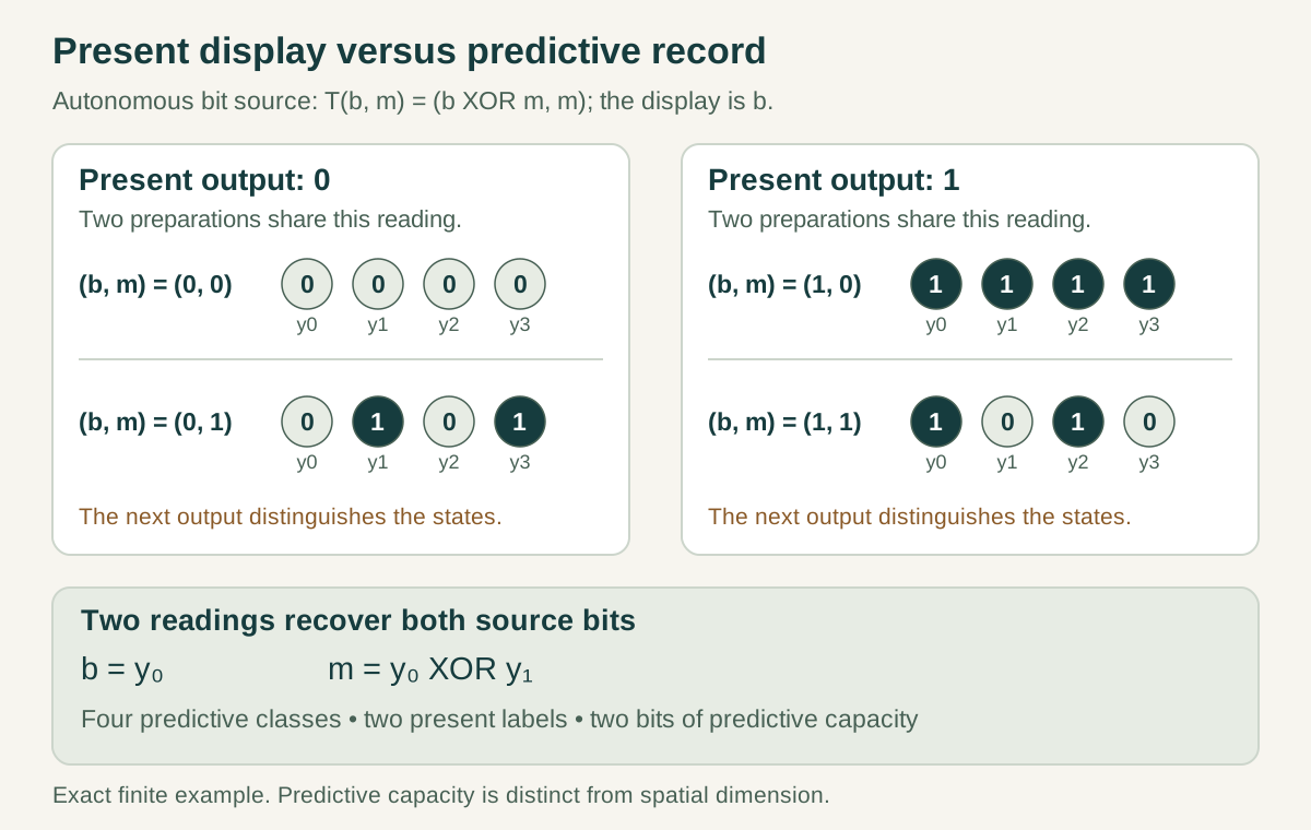
A DTT implementation can give the hidden bit a specific generative role. The new content lies in how that role constrains its update, access and cost, rather than in the mere existence of an unobserved variable.

What if the memory cannot fit into finitely many linear modes?

An exact delay y(t)=u(t−T), with T>0, has transfer function e^−sT. A finite linear time-invariant ordinary differential system has a rational transfer function. The exponential is not rational: along the positive real axis it decays faster than every inverse polynomial. Therefore an exact delay cannot be represented by finitely many such states over all inputs and times.

An ordinary one-time delay equation or an age-profile field still represents it. Finite approximations can match a restricted frequency range, with an explicit error and increasing memory cost. The result separates finite linear memory from exact delay; it does not prove a second measurable clock.

For the source programme, this suggests a useful resource question: how many retained states are needed to approximate a derived kernel over the physically accessible bandwidth?

Matching an unforced trajectory is not enough

Two source states can produce the same output while no control is applied and respond differently when a hidden coordinate is reset. An equivalence claim must therefore specify whether such a reset is physically available. If the auxiliary-state realization permits it, the age-field or dual-time description needs a corresponding operation; if neither permits it, it should not enter the comparison.

For the bit-swap example, the preparations (0,0) and (0,1) initially look identical. A control that sets the second bit to zero removes their future distinction. A control that only reads the first bit does not. The admitted operation changes which source information is predictively relevant.

A complete equivalence map includes these preparation and intervention rules as well as the evolution equation. This is a productive place for new dual-time content: a source law may constrain which resets or partial completions are physically realizable and at what resource cost.

A decaying kernel does not guarantee a stable system

Take ẋ=−x+z and ż=−z+2x. The memory kernel is 2e^−t, which decays, but the full evolution has eigenvalues −1±√2. One is positive, so some preparations grow. The feedback strength matters as well as the decay rate.

Thus a mathematical realization also needs the physical conditions appropriate to its use: bounded resources, stable or controlled growth, admissible preparations and, for quantum states, valid probability-preserving dynamics. A kernel fit alone does not certify these properties.

A strong contribution would provide both realizations, prove their equivalence for the admitted controls and determine their minimal retained information. It would then identify a joint source restriction—perhaps relating decay, completion and propagation—that survives the rewriting. That is where a temporal architecture can gain additional predictive content.

Continue reading

• When memory can be represented by one time →
• One source, retained memory and the construction of predictive records →
• Temporal asymmetry: geometry, memory, and reduction →
• Test predictive memory and repeatable completion →

Read this discussion as part of a path

• Meaning, explanation and distinction →