
Completed-future equivalence gives a precise predictive state. In a finite linear model its minimal size is the rank of a delay-observation matrix; discarded information appears as an exact memory term.
1. Specify the source before drawing its world
Begin with a state set S, a fixed update T:S→S and an output map R:S→Y. A preparation chooses s₀; subsequent states are sₖ=Tᵏs₀ and readable outputs are yₖ=R(sₖ). The state includes every register that can influence a later output. Calling one component “the source” does not permit controller memory or a retained archive to disappear from this description.
This is the smallest mathematical language needed to separate generative activity from completed observation. SMM motivates a common generative origin; DTT distinguishes the work producing an outcome from its availability as a record. Neither principle requires locating the source at an already existing spatial point. Spatial labels can instead be constructed from relationships between outputs.
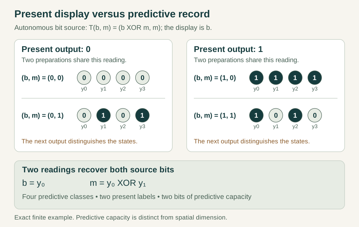
For a concrete model let S consist of two bits, s=(b,m), and define T(b,m)=(b XOR m,m), with R(b,m)=b. Here XOR means addition modulo two. The visible bit changes exactly when the retained memory bit is one. T is autonomous, reversible and completely specified: T² is the identity. It supplies one dynamics with four possible preparations and a one-bit display. A completed update is one application of T followed by the declared output operation.
The example is a logical realization, not a cosmological derivation. Its value is that claims about multiplicity, recurrence and memory can now be proved or refuted without ambiguous metaphors.
2. Derive the state seen by all completed future tests
Define two source states to be predictively equivalent when every allowed future observation agrees:
This relation is reflexive, symmetric and transitive because equality has those properties. It is also preserved by the update: if s∼t, replacing k by k+1 shows Ts∼Tt. Therefore T descends to a well-defined update on equivalence classes, [s]↦[Ts]. The output R also descends because the condition includes k=0.
The construction is maximal in a precise sense. Suppose another equivalence identifies states, preserves the output and is stable under T. Induction shows that equivalent states have identical outputs after every number of updates. That equivalence can therefore identify no pair that the completed-future relation separates. The resulting quotient is the coarsest deterministic state description retaining all admitted predictions.
If there are several allowed controls, replace Tᵏ by every finite permitted control word. Closure under appending a control supplies the same descent proof. Expanding the controls or detectors can only refine the quotient: more tests may separate previously indistinguishable histories. Thus “complete record” always refers to a specified operation language.
This is the operational role of completion in the published framework cited below. The proof does not assume a Hilbert space, a probability law or a physical clock. Those structures may be introduced later, with their own measurable meanings.
3. Four preparations, one display and two-step reconstruction
Apply the definition to the bit source. Starting from (0,0) gives 0000…; (1,0) gives 1111…; (0,1) gives 0101…; and (1,1) gives 1010…. All four future sequences differ. Consequently the predictive quotient has four classes even though the present display has only two values.
Two consecutive readings reconstruct the entire source state. One reading cannot: the preparations (0,0) and (0,1) both display zero, yet their next outputs differ. This gives both an upper bound and a lower bound on predictive memory. Two bits suffice to label the four states, and fewer than four deterministic labels cannot reproduce all four future sequences.
Under a uniform preparation ensemble, the full source entropy is two bits and the present output entropy is one bit. The remaining one bit is hidden conditional information. Those numbers refer to the specified ensemble; the cardinality argument needs no probabilities at all. A nonuniform preparation changes entropy without changing which states are distinguishable.
The model also clarifies persistence. When m=0 the visible label stays fixed; when m=1 it alternates. Both behaviours follow from retained state rather than repeated external instructions. A physical persistent object would require more, including a stable response to perturbations and appropriate conserved quantities, but the logical distinction between a continuing law and a replayed picture is already explicit.
4. Prove the autonomy criterion and its unavoidable error
For a finite linear source let V be a real inner-product space, M its completed update and P an orthogonal projection onto retained coordinates. Put Q=I−P. We seek a linear update B on PV such that PM=BP, so the next retained state depends only on the present retained state.
Necessity follows by multiplying on the right by Q: PMQ=BPQ=0. Conversely, if PMQ=0, then PM=PMP; choosing B as the restriction of PM to PV proves sufficiency. The criterion is therefore exact:
There is a useful quantitative extension. For every proposed B, restricting PM−BP to hidden inputs gives PMQ, so its operator norm cannot be smaller than ‖PMQ‖. The choice B=PM|PV achieves this lower bound. Hence the best possible one-step approximation error is exactly ‖PMQ‖. It measures how strongly discarded variations can re-enter the display.
For M(x,y)=(ax+by,cx+dy) and P(x,y)=(x,0), the residual is |b|. No clever update fitted only to x can remove this worst-case error over all admitted hidden preparations. Restricting y by a preparation rule can change the problem, but that restriction must be stated. This separates an actual predictive closure from a good fit on an unreported subset of states.
5. Recover minimal linear memory from delayed observations
A failed instantaneous projection does not require retaining every microscopic coordinate. Let the measured output be Cx, where C may have several rows, and let xₖ₊₁=Mxₖ on an n-dimensional real space. Stack successive readings into the observability matrix:
The semicolons mean vertical stacking. A state difference z is invisible through these n readings exactly when Oₙz=0. The Cayley–Hamilton identity expresses Mⁿ as a linear combination of lower powers. Multiplying by C and then by further powers of M shows that the same z is invisible at every later step. Thus ker Oₙ is precisely the subspace of differences invisible to all future outputs.
It is invariant under M: if z is forever invisible, then Cz, CMz, CM²z,… vanish, and the shifted sequence proves Mz is also invisible. Consequently V/ker Oₙ carries an autonomous predictive update. Its dimension is rank Oₙ by rank–nullity. Any linear state representation preserving all future outputs must retain at least this many independent distinctions.
For C=(1,0) and M=[[a,b],[c,d]], the first two readings have matrix [[1,0],[a,b]], whose determinant is b. When b≠0, they recover y₀=(x₁−ax₀)/b. For small |b| the reconstruction is noisy even though exact rank remains two. Predictive dimension and stable accessibility are therefore separate diagnostics, just as spatial rank and well-conditioned geometry are separate.
6. Calculate the memory created by discarding a coordinate
The same two-coordinate system yields a closed equation with delayed output. Write xₖ₊₁=axₖ+byₖ and yₖ₊₁=cxₖ+dyₖ. Substitute the second into the next x update and use byₖ=xₖ₊₁−axₖ. No division by b is needed in this algebraic identity:
The displayed coordinate has become a second-order recurrence. Its predictive initial data are two successive readings, or one reading plus the missing hidden information. If b=0, the original first-order recurrence already suffices; the second-order equation is then redundant and admits extra sequences unless its initial data satisfy the original restriction.
Take a=d=1/2 and b=c=1/4. The full eigenvalues are 3/4 and 1/4, so every state decays toward zero. The reduced equation is xₖ₊₂=xₖ₊₁−(3/16)xₖ. With x₀=0 and y₀=1, the observed sequence begins 0, 1/4, 1/4, 13/64. Omitting the hidden initial preparation would wrongly predict an identically zero sequence from x₀ alone.
This calculation complements the continuous memory-kernel example in the temporal-asymmetry guide. The memory is derived from elimination, not postulated afterward. Its existence establishes information loss in the reduced description; it does not independently establish a second laboratory clock, a thermodynamic entropy law or fundamental irreversibility.
7. Implement nested work and certify completion
A longer source episode may contain six nested inner roles. To model their execution autonomously, include an internal control pointer k, work registers w and retained archive a. Define one update F that advances the pointer and applies the operation prescribed at that pointer. Higher roles consume certified outputs of the lower ones. The outer role exposes a record only after the required dependencies have been completed.
This construction proves that one update can implement a nested process. Its explanatory content depends on the rules inside F. Arbitrarily programming six unrelated operations into a shared controller does not prove that geometry, clocks and matter must agree. A stronger construction derives their common restrictions from the same conserved quantities or admissible operation algebra.
Completion also needs a payload test. In a quantum realization, an accepted instrument of the form Iacc(ρ)=pVρV†, with V an isometry and p independent of ρ, preserves every admitted unknown input conditional on success. The probability is Tr Iacc(ρ)=p, and division by p leaves VρV†. The identity should remain true with an untouched reference system, since otherwise hidden correlations could be filtered.
If failed attempts restore the input and independent fresh trials succeed with probability p, the expected number of attempts is 1/p. At p=1/4, four attempts are required on average. A clock counting successful archives and a clock counting actual work therefore need an explicit conversion. The seventh role certifies availability; it does not make failure, retention and reset resources vanish.
8. Account for resources and compare rival source laws
The finite constructions suggest a practical ledger. Specify the number of accessible source states, the retained labels, the operation sequence, the allowed preparations and the output accuracy. Distinguishing K classical alternatives requires at least K reliable labels, equivalent to a capacity of log₂K bits. This is a capacity statement, not automatically the entropy of a particular ensemble or an energy cost for every update.
Then vary a hidden preparation while keeping its present display fixed. If a later permitted test separates the outputs, either enlarge the retained state or explicitly restrict the admitted test language. For linear dynamics, compute rank Oₙ and the smallest nonzero singular value of Oₙ. The former counts predictive coordinates; the latter bounds reconstruction sensitivity after units and noise norms have been chosen.
A shared-source theory becomes stronger when the same restriction predicts more than one interface. For example, a symmetry that suppresses PMQ may simultaneously constrain a clock response or a transport matrix. Demonstrating those linked consequences would remove an independent modelling choice. Merely setting two coefficients equal in the initial specification would demonstrate compatibility, not selection.
Compare a rival update with the same present outputs but different delayed outputs. The four-state source supplies the simplest such comparison. More realistic versions should keep the resources and preparation classes fixed. Otherwise an apparent advantage may come from supplying extra memory, calibration or control to only one model.
9. The SMM/DTT result and its next physical bridge
The constructive result is a route from source histories to the smallest state that preserves their observable futures. It supplies an exact quotient, a finite reconstruction method and a calculable obstruction when an instantaneous display forgets relevant information. These are positive mathematical structures with direct value for designing a source model.
For SMM, multiplicity belongs to distinguishable records and their relations, while unity belongs to the dynamical origin. For DTT, inner work can carry information not yet exposed by an outer record. Completion becomes scientifically useful when its retained state is sufficient for the next admitted experiments, rather than merely being declared complete by a narrative boundary.
The next bridge is a common source law that selects the memory, spatial operations and physical clock together. Its variables must have independently defined measurements; its predictions must survive changes of preparation without refitting an arbitrary interface. An admissible perturbation that changes memory should then induce a constrained, calculable change elsewhere.
The following chapter studies what happens when the retained outputs acquire paired spatial directions. The present analysis remains active there: a three-dimensional image may require a larger predictive state, and a completed archive may need information absent from its spatial coordinates. Keeping those distinctions explicit is how a generative account can gain physical content while preserving the rigorous results already available.
Continue with the articles
- From one source to many observable records
A common state can support coherent alternatives and many distinguishable records. An interference calculation shows why an SMM/DTT account must connect inner composition with outcome probabilities rather than assume classical alternatives.
- One action, two temporal roles
Inner generation and outer record order can be roles of one process. A completed return becomes an observable advance only when its action respects the retained records and their tests.
- When two histories count as the same observation
Completion identifies histories that leave the same record, while observation identifies records that available tests cannot distinguish. Their combined quotient is consistent only with the declared operations and contexts.
- Test languages and observable quotients
A test language determines which records an observer can distinguish. Enlarging that language refines the observable quotient and reveals when apparently different instruments retain the same information.
- Retained observations versus predictive states
A readable record need not contain enough information to predict its next update. An exact leakage criterion identifies when a linear completion is autonomous and measures the error when hidden information returns.
- A quantum source for generation and completion
A positive phase–dilation Hamiltonian ties one phase encoder to a powered coordinate and controlled work. It gives an explicit quantum realization of generation and completion while retaining its constitutive interfaces as inputs.
- Completion without biasing an unknown input
A factorized accepted channel gives the same success probability for every admitted unknown input, including inputs entangled with a reference. The failure channel and the amplification of errors by conditioning require separate checks.
- A record that carries its own completion certificate
An autonomous history Hamiltonian can generate both a data record and a flag tied to its completed write. The exact construction retains incomplete outcomes, coherent intermediate stages, and finite observation windows.
- What spatial readout forgets
Different inner states can share one spatial readout and still have different successors. A concrete counterexample and a kernel-preservation criterion identify the memory needed for autonomous completed evolution.
- Eliminating hidden variables creates memory
Eliminating a relaxing hidden sector yields an exact memory equation for the retained variables. The resulting kernel and initial-state term preserve causal dependence while exposing information absent from the current readout.
- Completion, commutants, and positive frequency
This guide follows completion, compatible complex structures and positive-frequency selection through their separate mathematical roles. Finite examples connect the framework to SMM/DTT while keeping causal readout and physical calibration as additional constructions.
- Temporal asymmetry: reading the published model
The temporal-asymmetry model connects projected dynamics with memory and path dependence. A solvable hidden-mode example distinguishes those effects from dissipative stability and from evidence for a second observable clock.