
Record sufficiency, payload recovery, fresh preparation and later retention are distinct conditions. Exact finite examples show how each can be checked without interpreting every memory effect as an additional clock.
Ask whether the same record permits different futures
Choose a declared current record and a fixed future intervention. Prepare two legal source states that produce the same present record. If their next-record distributions differ, the current record is insufficient for that prediction. This is an operational question about a test language, not a demand to observe every microscopic variable.
For probability distributions P and Q with total-variation distance δ, any predictor R using only the shared current record has error at least δ/2 on one preparation. The triangle inequality gives δ≤TV(P,R)+TV(R,Q). In the illustrative binary case with next-outcome probabilities 0.2 and 0.8, δ=0.6 and the unavoidable worst-case error is at least 0.3. These numbers define a mathematical witness, not experimental frequencies.
Calculate the hidden-to-visible part of an update
For a finite linear system, let P retain x and let Q=I−P retain the omitted coordinate y. An autonomous next-record map T exists exactly when PMQ=0. The necessary direction follows by multiplying PM=TP by Q; the sufficient direction follows from PM=PMP.
As an illustrative stable update, take M(x,y)=(x/2+y/4,y/2). Inputs (0,1) and (0,−1) have the same displayed zero, yet their next displays are 1/4 and −1/4. The norm of the hidden-to-visible block is 1/4, equal to the best possible operator-norm residual in approximating PM by TP. Retaining y restores an exact update. A smaller record can also work after a justified preparation restriction, but that restriction becomes part of the model.
A population record can omit predictive phase
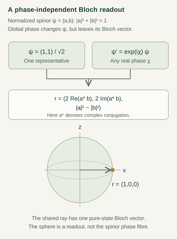
The states (|0⟩+|1⟩)/√2 and (|0⟩−|1⟩)/√2 have equal Z populations. Applying the same Hadamard gate makes their next Z outcomes certainly zero and certainly one. Thus a population record is insufficient for this continuation even though the full density operator predicts it exactly.
Open the full-size diagram →
The diagram distinguishes global phase, which the stated quadratic readout removes, from relative phase, which can determine a future population. Completion must specify which information is retained under the admitted operations. DTT can interpret the unreported distinction as generative memory; the calculation itself also has an ordinary one-time quantum-state description. That comparator keeps the positive information result separate from a claim about the number of physical time parameters.
Compare a memory equation with its one-time realization
Consider ẋ=−ax+by and ẏ=−λy+kx with λ>0. Solving the second equation and substituting gives a preparation term be−λty(0) plus a memory integral. Both arise from the same enlarged equations:
Choose a=2, λ=3 and b=k=1 in illustrative units. The system matrix has negative trace −5 and positive determinant five, so both eigenvalues have negative real part. This supplies a stable example with genuine reduced memory and one evolution parameter. Omitting y(0) would compare different preparations. A source theory adds predictive content by deriving the kernel or a relation to another observable, rather than by renaming this standard elimination.
Derive repeatability from the complete failure map
Let a complete instrument have Macc=√p V and Mfail=√(1−p)W with known unitaries. After recorded failure, W† restores the original payload. Fresh independent apparatus preparations with the same p then give the first-success law p(1−p)n−1. Stop applying the operation after success, so the work V is applied once.
For the declared illustration p=1/4 and K=20, the failure probability is (3/4)20≈0.003171, while the untruncated mean number of attempts is four. The average consumption and allocated worst-case capacity are different resources. Neither formula follows merely from seeing a stable average acceptance fraction.
For a capped run, expected activated attempts are Σk=1K(1−p)k−1=[1−(1−p)K]/p. At the same illustrative p and K this is about 3.9873, slightly below four because an exhausted run stops. A clock measuring all activated preparation and recovery operations must account for this cost; a record counting only successful work does not contain it automatically.
Check the stored result after the completion flag
A completion flag certifies a write only under its specified dynamics. Later readout tests whether the written label survives source evolution, environmental coupling and further use of the archive. Declare the delays, allowed disturbances and error statistic; do not identify successful writing with indefinite storage. Recovery quality and retention quality enter different parts of the operational account.
The SMM/DTT objective is one model relating the six nested generative dependencies to predictive state, accepted work and accessible memory. A useful result might bound all three with the same fixed coefficients. The record-memory guide supplies the exact closure criterion, while the registration-order guide tests a controllable way retained coherence changes later completion.
A useful retention comparison prepares the same accepted label with different earlier histories and applies identical later disturbances. If later errors depend on those histories, the stored label alone has not specified the memory state. That finding identifies which initialization or retained information must be added to make the next-readout law repeatable.
Continue with the articles
- Completion without biasing an unknown input
Explain the construction of a loaded completion channel with input-independent success probability. Clarify why this condition matters when the matter state is unknown.
- Reliable completion by repeated attempts
Explain the geometric success law for fresh, recoverable attempts and the finite-archive reliability bound. Relate reliability to resource budgets rather than an assumption of guaranteed completion.
- A phase-sensitive registration experiment
Outline the proposed protocol linking source coherence to later completion statistics. Compare its response matrix and energy diagnostic with a simpler qubit baseline.
- Eliminating hidden variables creates memory
Explain how removing the hidden sector produces an exact Volterra equation in the dual-time gauge model. A memory term can emerge even when the larger dynamics are specified locally in time.
- When memory can be represented by one time
Introduce finite Markovian embeddings of strictly proper real-rational memory. Explain why a hidden-memory description does not automatically imply an additional observable temporal degree of freedom.
- How a protocol can reveal dual-time structure
Outline ways to move beyond the finite prepared linear interface: protocol-dependent access, noncommuting transport, or richer memory. Each route must be defined as an observable procedure.