Validate a coupling through normalized response

Declare the probe as carefully as the receiver

Specify a finite real inner-product space of response variables F, a positive self-adjoint stiffness K and a nonzero source direction f. For Hermitian receiver variables, the inner product is tr(XY). The supplied energy is E(F)=⟨F,KF⟩/2 and the imposed scalar current is j=⟨f,F⟩.

Fix the normalization of f independently. A change of coordinates transporting the metric, stiffness and source together leaves physics unchanged; multiplying f alone changes what one unit of imposed current means. Likewise, doubling K with the probe held fixed changes the apparatus response. SMM/DTT seeks a common origin for these quantities in the generative receiver. Counting its completed records supplies only one part of the required specification.

Positivity is itself a validation requirement: a zero mode coupled to the imposed source can invalidate a finite inverse-capacity formula. Either restrict to a justified positive sector or analyze that mode explicitly before using K⁻¹.

Obtain the minimum and its unique field

A multiplier λ for the current constraint gives KF=λf, so F=λK⁻¹f. Inserting the constraint fixes λ=j/C, where C=⟨f,K⁻¹f⟩. The exact minimizer and minimum are:

To verify uniqueness, write any other admissible field as F_*+Z with ⟨f,Z⟩=0. The cross term in its energy vanishes because KF_* is proportional to f, and the remainder is ⟨Z,KZ⟩/2>0 unless Z=0. This is a positive exact result: one scalar capacity fully determines the minimized static current cost. It also identifies the information that this single measurement does not reveal about the internal field.

Compare equal dimensions with different responses

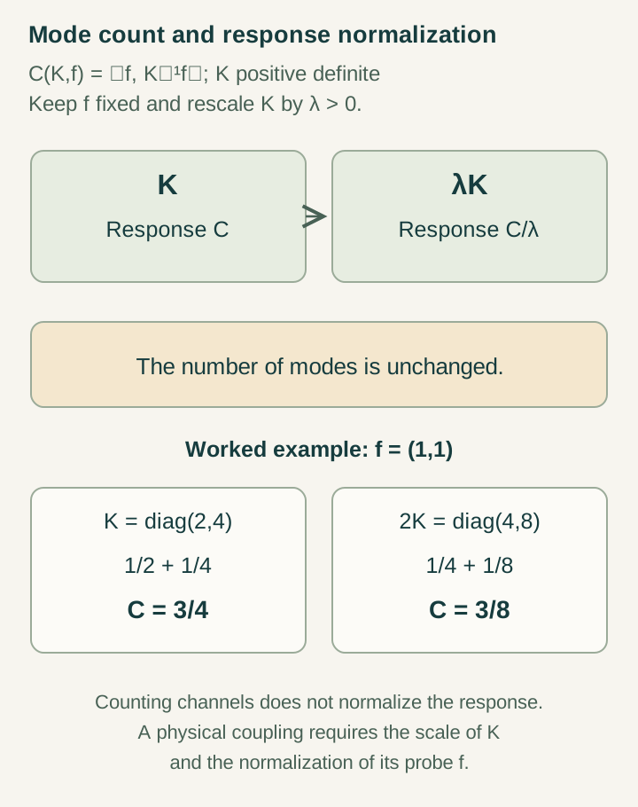
Choose the illustrative two-dimensional inputs K=diag(2,4), f=(1,1) and j=1. Then K⁻¹f=(1/2,1/4), C=3/4 and F_*=(2/3,1/3). Substitution gives E_min=[2(4/9)+4(1/9)]/2=2/3.

Now double K while retaining the source and current. Capacity becomes 3/8, the minimizing field stays (2/3,1/3), and the minimum energy doubles to 4/3. The receiver dimension remains two. Both are consistent positive response models, so dimension cannot select between them.

The figure depicts this exact scaling, not an observed susceptibility. A validation calculation should recover it before claiming that a more complicated source construction fixes a normalized interaction.

Allow unobserved directions to lower the cost

For ordinary trace coupling in rank N, set e₀=I_N/√N and write F=xe₀+Z with tr Z=0. The constraint fixes x=j/√N. In this decomposition let K have blocks [u, b†; b, D], where D is positive. Minimizing over the hidden directions gives Z_*=−xD⁻¹b and effective stiffness s=u−b†D⁻¹b.

With illustrative u=2, D=2 and b=1, s=3/2; the block has positive eigenvalues one and three. Freezing the hidden coordinate would instead use stiffness two and overestimate the cost. The completed trace response therefore depends on hidden relaxation even when the detector never separately reads the traceless sector.

Test what a 137-dimensional receiver actually fixes

Under the selected receiver grammar, sectors have ranks 100, 30 and seven. Assigning positive isotropic stiffnesses κ₁, κ₂, κ₃ gives C=100/κ₁+30/κ₂+7/κ₃. Equal coefficients yield 137/κ; doubling only the first yields 87/κ. Both retain the same available records and each sector’s internal unitary symmetry.

This comparison makes the missing law precise: a source construction must justify the relative response weights and their common scale. The structural ideal integer 137 is exact under its stated grammar and receiver assumptions. It is not the measured inverse fine-structure constant, and its sector count does not describe energy running. A matched coupling requires a physically normalized observable beyond the integer.

Form the dimensionless quantity in one shared convention

After a separately supplied three-dimensional continuum limit, the trace-response convention gives potential V(r)=−A_N/r with A_N=s_cont/(4πN). Match the same action scale a and propagation speed c used in the matter dynamics. The dimensionless result is g_N=s_cont/(4πacN).

The continuum coefficient s_cont has units of energy times length. A finite graph stiffness cannot be substituted without its scaling map. The ideal relation g_N=1/137 requires both N=137 and s_cont/(4πac)=1, followed by electromagnetic identification. The latter ratio cannot be set by changing units. It is exactly the response-to-matter relation that a stronger SMM/DTT source dynamics must derive.

Reserve an observable that can distinguish the models

Freeze the receiver, probe, continuum matching and action/clock dictionary. If one static capacity is used for calibration, calculate a second response with a separately normalized probe, a frequency dependence or a nonlinear coefficient. State which admissible models remain after the calibration and whether the new quantity is constant across them. More measurements of the identical scalar capacity improve precision without necessarily identifying internal rank.

The useful SMM/DTT connection is a restriction linking receiver construction, field response and matter propagation through six nested inner dependencies and one completion interface. Hydrogen can then test linked scales using the resulting coupling. It cannot select the coupling merely because binding occurs. The normalization problem records that bridge, and the atomic validation guide follows its conditional consequences.

For a simple second-probe illustration, keep K=diag(2,4) but use f′=(1,−1). Its capacity remains 3/4, while the cross-response ⟨f,K⁻¹f′⟩ is 1/4. The pair of probe directions accesses information unavailable in one scalar capacity. A different model agreeing on the first probe can be tested through this cross-response, provided both source normalizations and their relative orientation are independently fixed.

Continue with the articles

• Why a record count is not yet a coupling

  Explain why the static response depends on the source and inverse response operator, not simply on the number of records. This is the central bridge required by the coupling proposal.

• Trace-sector response and the Schur complement

  Introduce the reduction that gives capacity N/s under ordinary trace coupling. Show how hidden response sectors can affect an apparently simple scalar observable.

• The conditional ideal value one over 137

  Summarize the extra normalization and electromagnetic matching needed for the ideal model coupling. Explain why the draft’s alpha-zero notation does not denote the measured low-energy constant.

• A dependency map for physical constants

  Introduce the constants program as a chain from completion dynamics to response and then physical matching. Identify which quantities are structural, calibrated, or still free.

• Prediction after calibration

  Present the calibration-fiber criterion for a conditional prediction. An additional observable must be fixed across the allowed calibrated models to avoid merely reusing its target value.

• Why binding does not fix the coupling

  Introduce the dilation argument showing that a family of positive couplings remains compatible with binding and completion. Identify the extra source-selection law needed to obtain a specific interaction strength.