
A positive quadratic response has capacity C=⟨f,K⁻¹f⟩. Ordinary trace coupling gives C=N/s after hidden-sector relaxation, so a physical coupling contains both an inverse rank and a primitive normalization.
Which part of a completed record resists change?
In DTT, a public interaction should arise from the response of the same process that generates and completes spatial records. Imagine imposing a small source on a retained receiver. The source asks for an observable output; the inner field can distribute that request among available directions. Its least energy defines an effective stiffness visible at completion.
This question goes beyond counting records. Two receivers of equal dimension may assign different energetic costs to their modes. Conversely, different internal receivers may have the same net static response. The required mathematical objects are therefore a positive response operator, an independently normalized source and a rule relating their output to physical fields.
Derive the capacity by minimizing energy
Let F be a Hermitian receiver field with real inner product ⟨X,Y⟩=Tr(XY). Let K be positive and self-adjoint, and let f be the Hermitian source direction. The quadratic energy is E(F)=½⟨F,KF⟩. Fix the scalar current j=⟨f,F⟩.
A Lagrange multiplier gives KF=λf. Therefore F=λK⁻¹f and j=λC, where C is the source capacity. The unique minimizer and its cost follow immediately.
Emin=j²/(2C)
Uniqueness follows from positivity: adding any Z with ⟨f,Z⟩=0 makes the cross term vanish and adds ½⟨Z,KZ⟩. The operator K here is a stiffness, not the phase generator used elsewhere.
An exact example with the same 137 records
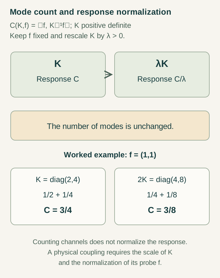
For ordinary trace coupling f=IN and isotropic stiffness K=κI, the capacity is N/κ. The structural receiver has sectors of ranks 100, 30 and 7. Giving them positive stiffnesses κ1, κ2 and κ3 yields a different but equally well-defined response.
Open the full-size diagram →
If all stiffnesses equal κ, C=137/κ. If κ1=2κ while the others remain κ, C=87/κ. The number of retained states has not changed. A derivation of the inverse-rank law must therefore explain the stiffness relation, not just preserve the receiver dimension or require frame covariance.
Where the physical normalization enters
On a supplied spatial graph, current conservation and the minimized edge energy produce a Laplacian response. A controlled three-dimensional continuum limit then supplies the inverse-distance Green function. With the stated flux convention, write the attractive potential as V(r)=−AN/r, where AN=scont/(4πN).
The continuum stiffness scont has units of energy times length, as does ac when a is an action scale and c a speed. Thus scont/(4πac) is a genuine dimensionless physical ratio. Setting it to one is a proposed source law, not a choice of units. Under that additional condition N=137 gives the ideal value gN=1/137.
Connect the coupling to the hydrogen speed statistic
Supply the nonrelativistic relative Hamiltonian H=−a²∇²/(2mred)−AN/r. Its ground energy is −mredAN²/(2a²). The Coulomb virial theorem gives ⟨p²⟩/(2mred)=−E1, so the relative root-mean-square speed obeys:
After electromagnetic matching, gN is the coupling denoted α. The electron speed about the center of mass has an additional factor mred/me. The mean velocity vector of the stationary ground state is zero. This calculation connects response and atomic motion consistently, but the coupling entered through the Hamiltonian; binding does not select its value.
The common-source result to pursue
A stronger SMM/DTT construction would derive the receiver, f, K, the continuum scaling and the matter action from one autonomous update. Its six nested inner roles should constrain these quantities together before outer completion. The decisive relation would fix the primitive response relative to the independently measured action and propagation scales.
The alpha workbench also contains a compact-phase response route. Fitting that route to α can select a completion parameter; a subsequently calculated nonlinear response is a conditional new output. Reconstructing the fitted α is not an independent prediction. The useful next test is an additional response or spectral observable that cannot be retuned while keeping the calibration fixed.
Continue with the articles
- Why a record count is not yet a coupling
Explain why the static response depends on the source and inverse response operator, not simply on the number of records. This is the central bridge required by the coupling proposal.
- Trace-sector response and the Schur complement
Introduce the reduction that gives capacity N/s under ordinary trace coupling. Show how hidden response sectors can affect an apparently simple scalar observable.
- The conditional ideal value one over 137
Summarize the extra normalization and electromagnetic matching needed for the ideal model coupling. Explain why the draft’s alpha-zero notation does not denote the measured low-energy constant.
- A flag-independent response without one fixed rotation action
Explain the draft’s distinction between covariantly transported response and a single fixed rotation representation. A useful invariant can survive even when a stronger representation requirement fails.
- A dependency map for physical constants
Introduce the constants program as a chain from completion dynamics to response and then physical matching. Identify which quantities are structural, calibrated, or still free.
- Prediction after calibration
Present the calibration-fiber criterion for a conditional prediction. An additional observable must be fixed across the allowed calibrated models to avoid merely reusing its target value.
- A normalizable hydrogen-like ground state
Introduce the lower-bound and bound-state results of the effective model. Explain how the supplied kinetic and potential rules produce a meaningful atomic test case.
- Why binding does not fix the coupling
Introduce the dilation argument showing that a family of positive couplings remains compatible with binding and completion. Identify the extra source-selection law needed to obtain a specific interaction strength.