Does a hydrogen spectrum test the source or only its effective model?

What does a hydrogen calculation actually test?

A bound state is a valuable benchmark because one supplied Hamiltonian ties together a wavefunction, a length, a momentum distribution and an energy. Recovering these relationships checks whether a proposed source response can be used consistently in matter dynamics. Establishing that the source itself selects the Hamiltonian is a further task.

Consider the three-dimensional nonrelativistic Coulomb model H=−ℏ²Δ/(2μ)−κ/r, with positive reduced mass μ and attraction coefficient κ. This discussion derives its simplest exact state directly. The supplied constants and the physical identification of the two constituents are inputs. The source-response-to-hydrogen route asks how these inputs can be linked to a common SMM/DTT mechanism.

Separating those roles makes the benchmark stronger. A successful atomic calculation can verify an interface without being presented as an independent derivation of the electromagnetic coupling or electron mass.

A complete ground-state calculation

Try the normalized radial state ψ(r)=(πa³)^−1/2e^−r/a, where a>0. Its normalization follows from 4π∫₀∞r²|ψ(r)|²dr=1. For r>0, Δψ=(1/a²−2/(ar))ψ. Substituting into Hψ leaves a constant term and a term proportional to 1/r.

The state is an eigenfunction precisely when a=ℏ²/(μκ), giving E₁=−μκ²/(2ℏ²). Its energy is also the ground energy: the Coulomb quadratic form can be factored into a nonnegative sum of first-order norms after subtracting E₁, with ψ annihilated by the corresponding radial-plus-directional first-order operator. Equivalently, minimizing the normalized exponential family reproduces the exact eigenstate, while positivity of that factorization establishes the lower bound beyond the trial family.

Explicitly, use D=∇+r̂/a. Integration by parts gives ∫|Dφ|²=∫|∇φ|²+a⁻²∫|φ|²−(2/a)∫|φ|²/r for suitable decaying states. Multiplying by ℏ²/(2μ) yields ⟨H⟩−E₁≥0 with the chosen a. This states the domain and boundary behavior needed for the calculation.

One dimensionless input ties together three scales

Define g=κ/(ℏc). The model then gives the characteristic length a=ℏ/(μcg), binding magnitude |E₁|=μc²g²/2 and root-mean-square relative speed v_rms=cg. The last relation follows from ⟨p²⟩=ℏ²/a². It describes a momentum-distribution scale, not a classical electron following a circular orbit.

If the supplied g is multiplied by t while μ,ℏ and c remain fixed, a is divided by t, v_rms is multiplied by t and the binding grows by t². These relationships provide a coherent check of a proposed response law.

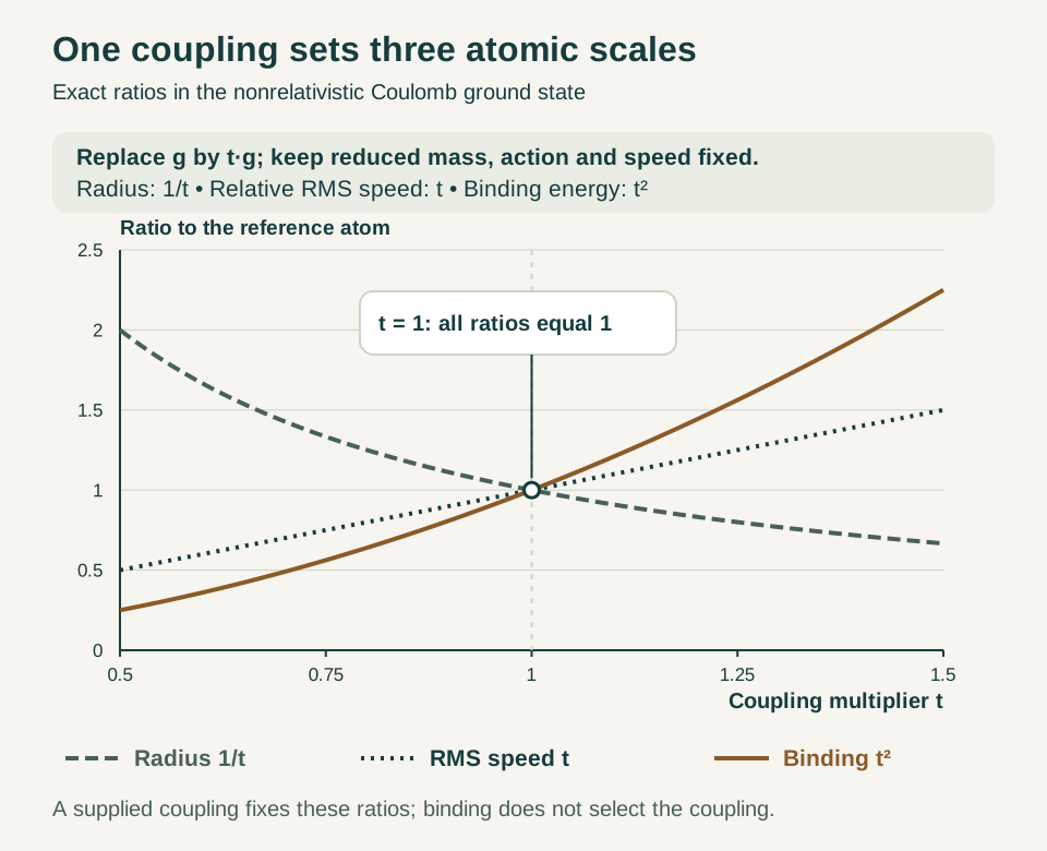
They also show why fitting one of these scales can determine the others within the assumed Coulomb model. That is a useful consistency relation, but it does not independently establish the microscopic origin of g.

When is the atomic calculation a new prediction?

Suppose the ground-state energy is used to infer g through g=√(2|E₁|/(μc²)). Inserting that same value back into E₁ reproduces the fitted energy identically. Predicting a or a second transition uses more of the model, but remains a test of the Hamiltonian after calibration.

A source-level prediction is stronger when the response calculation fixes g without atomic input, the matter construction fixes μ independently, and the resulting atomic outputs are held out. If g is inferred from one atomic measurement, the paper should say so and choose a genuinely independent comparison. The calibration discussion gives a general criterion: the predicted quantity must be fixed, or bounded, across all remaining admissible calibrated models.

The proposed ideal count 137 enters only after a normalized law identifies g with its reciprocal or with a corrected expression. The Coulomb solution accepts any positive κ; its mathematical existence does not select 137.

Why changing the nucleus is informative

For constituent masses m and M, the two-body separation coordinate has reduced mass μ=mM/(m+M). This follows by rewriting the kinetic energy in centre-of-mass and relative coordinates. With the same κ, the Coulomb binding is proportional to μ and the characteristic length inversely proportional to it.

For an illustrative mass choice M=9m, μ=0.9m; for M=19m, μ=0.95m. The binding ratio is 19/18 and the length ratio is 18/19 when the other inputs are shared. These are exact model numbers, not claimed isotope measurements. They show how a common response can be tested across two matter preparations without selecting a new coupling for each.

A realistic comparison must also include the nucleus’s charge distribution and whatever relativistic, radiative or structural terms are relevant to the stated precision. The hydrogen and deuterium guide organizes these as distinct inputs and comparison channels.

Different radius measurements answer different questions

The parameter a in the exponential state is a length scale, not every possible definition of atomic radius. Its probability density per unit volume is largest at the origin. The radial probability density, which includes the factor 4πr², is largest at r=a. Direct integration gives ⟨r⟩=3a/2 and ⟨r²⟩=3a².

These distinctions matter when a source’s completed spatial extent is compared with an atomic observable. A count of visited sites, a radial expectation and a form-factor scale require their own measurement maps. Agreement of one chosen “radius” cannot be assumed to imply agreement of all of them.

A controlled perturbation gives a further check. Add a weak potential δV(r)=λe^−r/R with fixed R>0. Its first-order ground-energy shift is λ⟨e^−r/R⟩=λ[1+a/(2R)]⁻³, obtained from the same normalized radial integral. This is a calculable response to a specified perturbation. A source model would need to derive λ and R independently before this becomes its new atomic prediction.

A useful next calculation for SMM/DTT

Specify a finite source that produces a positive static response and an effective matter kinetic term under one action–clock calibration. Derive the effective κ and μ and state the approximation that turns the source into the Coulomb Hamiltonian. Then vary a source parameter or a constituent preparation and calculate at least two linked atomic quantities with no new fit.

The deliverable should include the effective Hamiltonian, the state normalization, an error estimate for the reduction and a table identifying every calibration input. This gives mathematical physicists a tractable interface problem and atomic theorists a clear comparison. It also locates any missing ingredient: response normalization, mass selection, relativistic completion or the treatment of composite records.

Continue reading

• From a normalized source response to a hydrogen-like atom →
• A normalizable hydrogen-like ground state →
• Why binding does not fix the coupling →
• Hydrogen and deuterium as complementary probes →

Read this discussion as part of a path

• From structural counts to physical constants →