
The Coulomb model yields exact linked atomic consequences for every supplied positive coupling. A source-derived coupling would make these consequences predictions; binding alone does not select its value, and a stationary wavefunction is not yet a preparation mechanism.
1. Reduce the two-body problem in one physical convention
Supply two positive masses me and M, a common action scale a, and a positive attractive coefficient C. Let r=xe−xN be their separation and R=(mexe+MxN)/(me+M) their center of mass. The corresponding momenta separate the kinetic energy into P²/[2(me+M)]+p²/(2μ), where μ=meM/(me+M).
The relative problem is H=p²/(2μ)−C/r on L²(ℝ³), with p=−ia∇. Set D=a²/(2μ), so H=−DΔ−C/r. The scalar state space, Euclidean continuum, probability rule and local kinetic operator are explicit inputs. Their common origin is the source-reconstruction target; they are not supplied merely by naming a completed configuration an atom.
The previous chapter gives C=scont/(4πN) in its stated flux convention. Define g=C/(ac), using the propagation speed c and the same action scale a. Electromagnetic matching identifies a with ℏ and g with α after source and charge conventions are fixed. For an ideal structural model, g₀=1/137 remains conditional on the primitive response law.
With the potential zero at infinite separation, zero is the dissociation threshold. A normalized state of negative energy establishes binding in this operator. The question can now be solved without postulating an electron orbit or guessing a radius from a delay.
2. Prove the ground state globally
Use the quadratic form q[ψ]=D∫|∇ψ|²−C∫|ψ|²/r on H¹(ℝ³). The Coulomb singularity is controlled by the three-dimensional Hardy inequality: ∫|ψ|²/r≤2‖ψ‖₂‖∇ψ‖₂. Applying the elementary inequality 2uv≤εu²+v²/ε shows that the attraction is infinitesimally form-bounded relative to the kinetic term. The form therefore defines the usual lower-bounded self-adjoint Coulomb realization.
Choose the length b=2D/C. For smooth admissible states, expand |∇ψ+r̂ψ/b|². Integration by parts changes its cross term into −(2/b)∫|ψ|²/r because ∇·r̂=2/r. The flux at the origin tends to zero, so this identity introduces no delta function. Extension by form continuity gives:
Every normalized state therefore has energy at least −D/b². The function ψ proportional to exp(−r/b) makes the square vanish and attains the bound. Its exact ground energy is E₁=−C²/(4D). Equality forces exp(r/b)ψ to be constant almost everywhere, proving uniqueness of the scalar spatial ground state up to a constant phase.
This proof does more than optimize a trial orbit. It bounds all states in the form domain, including nonspherical ones, and identifies the state saturating that bound. Additional spin or carrier labels would belong to a separately declared state space.
3. Normalize the retained spatial record and its errors
The integral ∫₀∞rⁿe−λrdr=n!/λn+1 gives ψ₁(r)=e−r/b/√(πb³). The density per unit volume peaks at the origin, while the radial probability P(r)=4r²e−2r/b/b³ peaks at r=b. The shell factor r² explains the difference; neither peak defines a particle trajectory.
The same integrals yield ⟨1/r⟩=1/b, ⟨r⟩=3b/2 and ⟨r²⟩=3b². Thus the radial variance is 3b²/4. Because |∇ψ₁|²=|ψ₁|²/b², the kinetic energy is D/b² and the potential expectation is −C/b=−2D/b². The virial balance 2T+V=0 and total energy E₁=−T follow directly.
A finite source simulation can use an exact tail benchmark. Integrating the radial density beyond a boundary R gives:
At R=5b the omitted probability is 61e−10≈0.00277; at R=8b it is 145e−16≈0.0000163. These are analytic model values, not experimental uncertainty claims. A numerical implementation should separately track this boundary truncation, its spatial discretization and its state-preparation error. Agreement on the ground energy alone does not verify the retained probability distribution.
4. Derive the linked scale relations
Insert D=a²/(2μ) and C=gac. The atomic length and binding energy become b=a/(μcg) and B=|E₁|=μc²g²/2. Set x=r/b and write ψ(r)=b−3/2ϕ(x). This is a unitary change of length scale. Dividing the Hamiltonian by B gives the universal dimensionless operator −Δx−2/x.
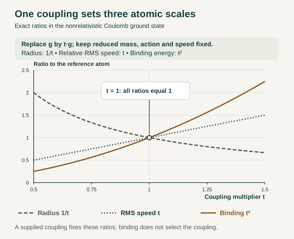
Consequently every positive g has the same normalized dimensionless ground profile while its physical radius changes as g⁻¹ and its binding magnitude as g². This demonstrates constructively why binding cannot select one coupling. The family is linked by exact dilations; changing g does not destroy its normalized ground state.
These relations become useful tests when the kinetic coefficient is fixed independently. For example, a source calculation that predicts b then also fixes B through the first identity. Permitting separate arbitrary energy and length conversions would erase that test. A common clock and action dictionary must connect phase evolution, energy and spatial readout.
The figure compares the consequences of multiplying g by a factor t with μ, a and c fixed. It plots exact ratios rather than measured atomic data. A perturbation to one source coefficient moves several observables together; that linked motion is more informative than a single matched radius.
Open the full-size diagram →
5. Define the speed and distinguish it from current
The velocity operator of the relative coordinate is v=(i/a)[H,r]=p/μ, using the conventional complex unit. Its RMS magnitude is √⟨p²⟩/μ. The ground-state gradient gives ⟨p²⟩=a²/b² and therefore:
The wavefunction may be chosen real, so its probability current j=(a/μ)Im(ψ*∇ψ) vanishes. Spherical symmetry also gives ⟨p⟩=0, while each Cartesian variance is a²/(3b²). A nonzero RMS magnitude is consistent with zero mean vector and zero current. It does not describe a hidden circular track or a measured orbital period.
The electron position is xe=R+[M/(me+M)]r. In the center-of-mass frame its velocity is p/me, rather than p/μ. Hence ve,rms/c=(μ/me)g and vN,rms/c=(μ/M)g. For equal masses each constituent has half the relative RMS speed. Only an infinitely heavy nucleus removes the electron's reduced-mass factor.
After electromagnetic matching, the relative ground-state relation is vrel,rms/c=α. The formula belongs to the nonrelativistic Coulomb model. It neither imposes a hard upper bound on every momentum measurement nor derives α from the existence of an atom. A DTT interpretation of source advances must recover this precise retained velocity statistic under the same kinetic operator.
6. Work one ideal example and a mass comparison
Choose declared model inputs N=137, gprim=1 and M=2000me. They imply g₀=1/137 and μ/me=2000/2001. These are illustrative choices, not empirical values of the nuclear mass ratio or a determination of the measured fine-structure constant.
| Quantity | Exact value | Approximation |
|---|---|---|
| Relative RMS speed divided by c | 1/137 | 0.00729927 |
| Electron COM RMS speed divided by c | 2000/(2001·137) | 0.00729562 |
| Binding divided by μc² | 1/(2·137²) | 0.0000266397 |
| Radius divided by a/(μc) | 137 | 137 |
Now double the illustrative nuclear mass to 4000me while holding the electronic coupling fixed. The reduced-mass ratio becomes μ′/μ=4002/4001. Binding increases by that factor, the atomic length decreases by its reciprocal, and the relative RMS ratio remains exactly 1/137. The electron COM speed changes with μ/me. This gives several different mass dependences from one two-body reduction.
Using the Coulomb spectral result En=−B/n², the first two adjacent intervals are 3B/4 and 5B/36, with ratio 5/27. The corresponding ordinary frequencies are ΔE/(2πa), while angular frequencies are ΔE/a. This spectrum is an additional exact result of the same Coulomb operator; the ground-state square proof alone does not derive every excited level.
These dimensionless ratios provide benchmarks before spin, radiation and nuclear structure are introduced. They do not specify transition intensities, lifetimes or precision spectral corrections.
7. Calculate a correction with a declared operator
A proposed source correction becomes meaningful when it changes an operator, rather than merely appending a small decimal remainder to 137. For a simple example add δV(r)=ηe−r/L/r, with fixed length L>0 and small coefficient η of dimensions energy times length. Its sign determines whether the added term weakens or strengthens attraction. This is a model perturbation, not a claimed SMM/DTT prediction.
For the isolated scalar ground eigenvalue, first-order perturbation theory gives δE₁=⟨ψ₁,δVψ₁⟩. Using the normalized radial state reduces the integral to 4ηb−3∫₀∞r exp[−(2/b+1/L)r]dr. Therefore:
δE₁/B=(8η/C)/(2+b/L)²
When L is much larger than b, the correction tends to η/b, as expected for an added η/r term. At L=b the normalized shift is 8η/(9C). When L is much smaller than b it is suppressed by (L/b)². The same length therefore leads to different relative effects across atoms or states with different characteristic sizes.
This example shows what a constructive holonomy or completion correction must supply: the operator, its coefficient, its scale dependence and a rule fixing those inputs before comparison. A perturbation also changes the state, so its corrected radius and momentum cannot generally be obtained by changing the energy alone. Higher-order terms require their own estimates, and a source-derived perturbation must respect the declared symmetries and shared physical dictionary.
8. Give completion a probability and a resource target
Unitary evolution leaves energy populations fixed, so an existing ground eigenstate is not a mechanism that prepares arbitrary inputs. A mathematically controlled selection instrument is Ks=exp[−s(H−E₁)] with s>0 of units inverse energy. Because H−E₁≥0, this is a contraction. The complementary operator Rs=√(I−Ks²) completes a two-outcome instrument.
If the initial pure state has ground probability p>0 and the spectral gap above E₁ is Δ, m consecutive accepted applications give a total success probability Pm between p and p+(1−p)e−2msΔ. The conditional ground fidelity is Fm=p/Pm, so 1−Fm≤[(1−p)/p]e−2msΔ. The inequalities follow by applying the spectral bound to the excited component while leaving the ground component unchanged.
For Coulomb Δ=3B/4. If p=1/4 and the excited component lies at the first excited energy, choosing msΔ=3 gives Pm=1/4+(3/4)e−6≈0.25186 and Fm≈0.99262. High accepted fidelity accompanies a success probability close to one quarter. If p=0, the filter never creates a ground component.
The isometry ψ↦Ksψ⊗|accept⟩+Rsψ⊗|reject⟩ explicitly retains both outcomes. An autonomous DTT mechanism must further supply its local implementation, initialized register, handling of failures, energy exchange and observable duration. The filter parameter s cannot simply be relabeled a physical clock reading.
9. Make the atomic benchmark a joint source requirement
The positive result now includes a global lower bound, a unique normalized scalar ground mode, an exact radial distribution, a momentum statistic, correlated scale relations and a normalized completion instrument. Each follows from declared mathematical inputs, and each can be checked against a finite source realization.
For SMM, a bound state can represent persistent organization produced by one source. DTT adds a specific dependency structure: six nested inner roles build what the seventh, outer completion makes accessible. The atom calculation becomes explanatory when those dependencies produce the same kinetic operator, mediator response, probability rule and clock used throughout the chapter. Assigning these independently and placing them under one controller would still leave their agreement unexplained.
A useful next theorem could control convergence from a finite retained graph to the Coulomb form, with the same coefficients governing propagation and response. Another could bound preparation error, success probability and physical duration together. A full coupling derivation would additionally fix g upstream, without using the atomic radius or line selected for comparison.
Once that upstream law is established, hydrogen supplies multiple consequences without new tuning. Corrections should then be introduced as explicit operators, compared across states and masses, and evaluated with the corresponding changes in observables. The atomic scale guide and isotope comparison provide organized checks. The exact identity connecting α and relative RMS motion is a valuable part of this chain because it joins response and matter dynamics in one calculation.
Continue with the articles
- A normalizable hydrogen-like ground state
Square completion gives the exact normalized ground state of the supplied nonrelativistic Coulomb Hamiltonian. Its spectrum and relative root-mean-square speed provide precise atomic benchmarks without selecting the coupling itself.
- Why binding does not fix the coupling
Dilation shows that every positive Coulomb coupling admits binding and the same type of ground-state filter. A source derivation of a particular coupling must therefore fix field, matter, action and clock normalization beyond the existence of an atom.
- Hydrogen fine structure and its temporal interpretation
The standard fine-structure Hamiltonian gives a quantitative benchmark for a temporal account of spin and relativistic transport. Its shared coefficients and n=2 splitting specify what a source model must reproduce before proposing additional shifts.
- State-dependent record cycles in hydrogen
A state-dependent record cycle needs a specified transport, physical band, phase convention and energy map. Shared level shifts then enforce transition-cycle consistency, which a separate adjustable phase for each line can violate.
- Hydrogen and deuterium as complementary probes
Hydrogen and deuterium separate universal electronic rules from isotope-specific mass and nuclear effects. Reduced-mass and contact-scaling examples show why a common operator can still produce different numerical shifts in the two atoms.