
Endpoint frame changes cancel around an Abelian loop. The resulting invariant is a possible comparison observable, while a group choice, field dynamics and physical detector require further input.
What you will learn
- Apply the endpoint rule for a local phase-frame change.
- Calculate a loop phase and show its invariance.
- Distinguish an invariant mathematical quantity from an accessible measured response.
Before you begin: Lessons 01–08, especially circular phase and quantum registration. Angles may be calculated in degrees in the worked examples.
Ask what a transformation preserves
A symmetry is described relative to data it preserves. Rotating a Euclidean vector preserves its length; permuting labels can preserve a graph. A change of basis instead changes the description of the same represented object. In a physical problem, specify whether a transformation acts on the system, the observer or the coordinates before drawing conclusions from the word symmetry.
Gauge freedom concerns local choices of representation. Different record locations can carry phase-bearing states without a preferred common phase convention. A transport rule tells us how to compare them. For SMM/DTT, this is a concrete way to ask how completed records share relational phase information even when their individual local labels depend on convention.
Derive the link transformation
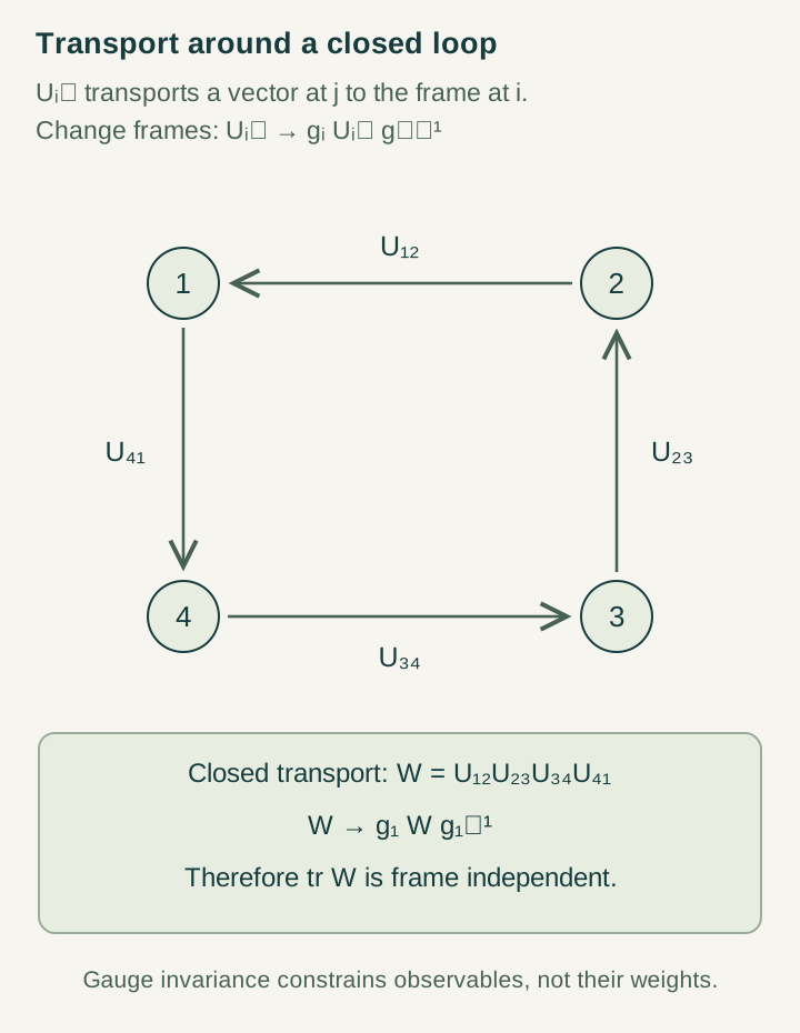
At vertex j let a component transform as ψ′j=exp(iχj)ψj. A link Uj=exp(iαj) carries the component from j to j+1. For the transported result to transform in the arrival frame, the new link must obey U′j=exp(iχj+1)Ujexp(−iχj).
The two extra terms refer to the endpoint conventions. They do not represent a new physical rotation applied to the carrier. Changing an actual link phase while holding frames fixed is a different operation. A calculation becomes interpretable only after this distinction between transport data and their local representation is kept explicit.
Worked example: four links close the path
Use the gauge-holonomy demonstration with link angles 30,45,−15 and 60 degrees. Their sum is Φ=120 degrees. The loop product is W=exp(iΦ), so its real part is −1/2 and its imaginary part is √3/2. In the one-dimensional U(1) representation its trace is simply this same complex number.
Change only the first frame to χ1=30 degrees. The first link becomes zero and the fourth becomes 90; the middle two remain 45 and −15. Their sum is still 120. Algebraically all frame terms cancel in the closed sum because each vertex appears once as an arrival and once as a departure. This is exact cancellation, not averaging over uncertain frames.
Open the full-size diagram →
Make the phase relative to a reference
A global phase multiplying a single isolated state leaves its density matrix unchanged. To observe the loop phase, supply a coherent reference. In an ideal balanced two-arm comparison, one arm acquires exp(iΦ) while the other does not. Recombination gives plus-port probability P+=(1+cosΦ)/2.
For the worked loop, cos120°=−1/2, giving P+=1/4. This is a concrete detector prediction under the additional interferometer assumptions. Reading cosΦ alone cannot separate Φ from −Φ; another phase setting can recover the missing quadrature. If path coherence is lost, the ideal fringe disappears. Thus gauge invariance identifies suitable information, while preparation and readout decide whether the experiment can actually access it.
What survives for matrix-valued transport
For higher-dimensional carriers, links are matrices and their order matters. Around a loop based at v, a frame change hv transforms the product as W′=hvWhv−1. The trace and eigenvalues survive conjugation even though individual entries change. The identity follows by cancellation of adjacent endpoint transformations in the ordered product.
This calculation does not determine which gauge group nature uses, what action governs its fields or what sets its coupling. Those are dynamical and physical selection questions. Likewise, invariance alone supplies no Yang–Mills mass-gap result. A source reconstruction must derive its carrier, admissible comparisons and dynamics before importing conclusions from a more specific gauge theory.
Connect the loop to a source protocol
A loop may be a path through spatial records or a controlled cycle in parameter space. A DTT interpretation must say which, then derive the corresponding transport from its source update. The six nested roles can organize dependent operations; their number alone does not assign an angle to the completed loop.
Design a useful comparison by fixing the source preparation, varying a declared loop protocol and retaining an independently defined detector output. Include a control where the effect vanishes. The holonomy guide gives an example of structure hidden in an inaccessible sector, reinforcing Lesson 03's test-language principle. Next we use a specified interaction to build a quantitative matter example: a bound Coulomb state.
Try the exercises
Work through each question, then open the answer to compare the steps.
Exercise 1
For link angles (10,20,30,40) degrees and vertex frame shifts (5,−5,10,0), calculate every transformed link and the loop sum.
Show the worked answer
Use arrival shift minus departure shift. The links become 10−5−5=0, 20+10−(−5)=35, 30+0−10=20 and 40+5−0=45 degrees. The transformed sum is 0+35+20+45=100 degrees, equal to the original 10+20+30+40. Every frame shift has cancelled once positively and once negatively.
Exercise 2
An ideal balanced interferometer measures a loop with Φ=60 degrees. Find its plus-port probability. Would measuring only that probability distinguish Φ=−60 degrees?
Show the worked answer
The probability is (1+cos60°)/2=(1+1/2)/2=3/4. Since cos(−60°)=cos60°, the same port probability occurs for the opposite phase. A second reference-phase setting sensitive to sinΦ can distinguish the signs. This illustrates why one invariant response need not retain every distinction contained in the full complex holonomy.
Continue with the articles
- Relational transport and gauge freedom
Explain why independently unframed record fibers require a rule for comparison. Introduce gauge transport as a conditional reconstruction idea, distinct from the draft’s exact Hamiltonian results.
- An exact singlet-loop response
Introduce the four-position mobile carrier and stationary dual used in the solvable model. Explain how the holonomy-dependent resolvent determines the ground-state response under the supplied Hamiltonian.
- Invisible holonomy in inaccessible sectors
Explain the draft’s classification of residual parallel monodromy invisible to the prepared interface. Nontrivial structure can survive outside the behavior an experiment can access.