
A specified receiver grammar yields 137 exactly. A coupling additionally depends on the response operator, source normalization, and identification with the matter interaction.
Read the earlier proposal through its dependencies
A Combinatorial–Geometric Derivation of the Fine-Structure Constant from Inner-Time Projection Dynamics in the Duality of Time Theory is a public preprint. Its abstract connects dimensional projection with an ideal inverse value of 137 and discusses corrections. This guide expands A212 while keeping the integer construction separate from its electromagnetic interpretation.
The ideal label α₀=1/137 is not automatically a bare coupling, a low-energy coupling, or a coupling at some high-energy scale. Such identifications need a specified physical theory, observable, and matching prescription.
Why a quadratic receiver has ten components
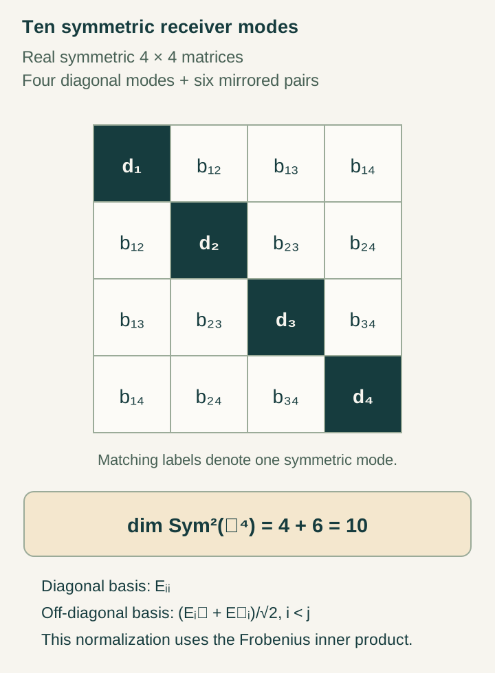
A four-dimensional input has four square terms and six unordered mixed pairs in its free symmetric quadratic receiver. Therefore dim Sym²(V)=4·5/2=10, over either the real or complex field when dimensions are counted consistently over that field.
This provides a structural origin for a factor of ten without appealing to decimal notation. It does not select the receiver automatically: why quadratic observables, why a four-component envelope, and which relations among the components are physically imposed? Those questions determine whether the free dimension is the relevant retained count.
Open the full-size diagram →
Calculate the retained count
The nonempty subsets of a d-element set number 2d−1. If a chosen record rule gives every old record ten extensions and adds one record for every new nonempty subset, the recurrence is Q₀=0 and Qd=10Qd−1+(2d−1).
The result is exact for that grammar. The rule for extending old records, admitting new branches, and stopping at depth three is substantive. A necessity argument must derive those rules from source operations and completion requirements rather than choose them after recognizing the target integer.
Count and capacity can vary independently
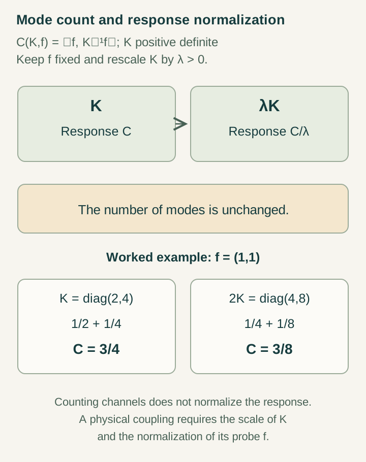
Let a positive receiver operator K respond to a source f with capacity C=⟨f,K−1f⟩. If K=sI and ||f||²=137, then C=137/s. The receiver dimension remains unchanged while its response varies with the positive stiffness s.
A physical derivation of α₀ would have to fix s and the source norm by the same construction, then prove the electromagnetic coupling is the appropriate inverse capacity. This is where the geometric count meets dynamics. A field redefinition cannot settle the issue unless the corresponding matter normalization is tracked as well.
Open the full-size diagram →
What the atom tells us once coupling is supplied
For the nonrelativistic Coulomb Hamiltonian with reduced mass μ and potential −αℏc/r, E₁=−μα²c²/2. The virial relation gives ⟨p²⟩/(2μ)=μα²c²/2, so the relative root-mean-square speed is sqrt(⟨p²⟩)/μ=αc.
In the center-of-mass frame, the electron speed is instead (μ/me)αc. Substituting α₀=1/137 yields the ideal model prediction after the coupling has been supplied. Binding exists for a continuous family of positive α values, so the existence of hydrogen-like binding does not by itself select 137.
Connect the structural and physical programs
Read A212 with A87–A90 and A96–A99. Then follow A171–A176 to see what is needed for attraction, a Coulomb law, and a normalizable atom. The strongest SMM/DTT objective is one source that fixes both the receiver and the matter probing it.
A useful next result would show that an allowed rescaling of K necessarily changes another already fixed observable, removing the free matching parameter. Only afterward should a fractional correction be calculated from a defined mechanism. Which response and atomic observations remain predictions after calibration? That question tests whether the integer has become a coupling explanation.
Continue with the articles
- The earlier combinatorial fine-structure proposal
Read the earlier coupling proposal alongside the newer response-based draft. Track the shift from structural counting to an explicit source, response operator, and electromagnetic normalization.
- From three-dimensional readout to retained records
Trace the latest draft’s route from quaternionic readout to a selected grammar with 137 distinguishable records. Keep each structural choice visible in the explanation.
- Why a record count is not yet a coupling
Explain why the static response depends on the source and inverse response operator, not simply on the number of records. This is the central bridge required by the coupling proposal.
- Trace-sector response and the Schur complement
Introduce the reduction that gives capacity N/s under ordinary trace coupling. Show how hidden response sectors can affect an apparently simple scalar observable.
- The conditional ideal value one over 137
Summarize the extra normalization and electromagnetic matching needed for the ideal model coupling. Explain why the draft’s alpha-zero notation does not denote the measured low-energy constant.
- Why the symmetric receiver has ten modes
Count the independent symmetric quadratic combinations of a four-component envelope. Explain the receiver interpretation and why selecting that construction is a substantive modeling choice.
- Alternating branches and the ranks one, three, seven
Explain how positive-degree exterior sectors produce the branch counts used by the reconstruction. Keep the counting argument separate from any identification with particle families.
- A normalizable hydrogen-like ground state
Introduce the lower-bound and bound-state results of the effective model. Explain how the supplied kinetic and potential rules produce a meaningful atomic test case.
- Why binding does not fix the coupling
Introduce the dilation argument showing that a family of positive couplings remains compatible with binding and completion. Identify the extra source-selection law needed to obtain a specific interaction strength.
Sources and reading
Read the original source for its exact formulation and edition. The examples on this page are explanatory reconstructions.