


Separate fitting from testing
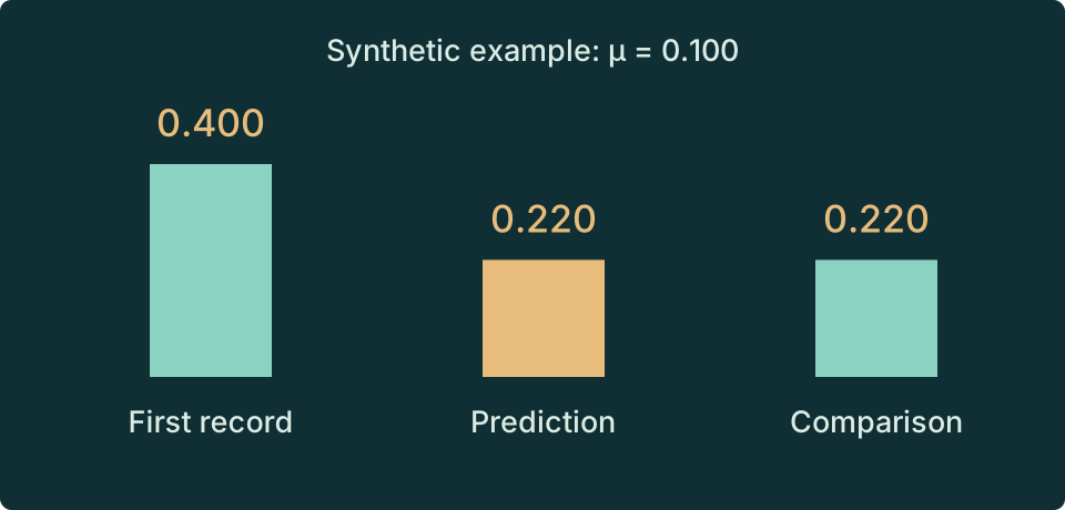
A model becomes more informative when a stated input fixes a result that was not used to choose that input. Here we use the first completed centre weight to determine μ, then predict the centre weight after a second update. This is a small example of parameter fitting followed by a held-out check.
The observations in this lab are synthetic demonstration values. They are editable numbers for learning the logic of comparison, not experimental measurements of Duality of Time Theory. A successful match verifies the supplied finite model against those numbers; it does not establish a physical interpretation. The research programme separates postulates, conditional results, physical identifications, and empirical predictions. [B16] [P01]
The example is deliberately simple enough to calculate without running the animation. That makes the visualisation accountable to a formula rather than allowing the picture to carry the argument by itself.
Fit once; compare the next record
The default first-step centre value is 0.400, giving μ = 0.100. The predicted second-step centre value is 0.220. Change the held-out value alone: the fitted μ and prediction stay fixed, while the residual changes.
Explore · teaching model v1
Teal: generated values. Gold: highlighted readout or reference.
Enable JavaScript to explore this model. The figure, worked values, and equations explain the same construction.
Export JSON to retain the assumptions, inputs, predicted values, and residual, or CSV for a 0–20-step centre-weight series. Exports explicitly identify the model and the synthetic nature of the comparison. They contain no browser history or account information.
Derive the two-step prediction
At the centre, six edges carry weight away from a unit seed. After one update the centre has weight 1−6μ and each neighbour has weight μ. All other sites still have zero weight.
At the second update, the centre retains a fraction 1−6μ of its previous weight and receives μ times the weight at each of its six neighbours. For μ = 0.1, the two contributions are 0.16 and 0.06, giving 0.22. Boundary effects do not change this centre calculation.
The allowed first-step value is between zero and one, which gives μ between 1/6 and zero. An external measurement outside that range would be inconsistent with this model and normalization. The lab constrains inputs to the admissible range; a research tool should retain out-of-range observations and report the failure rather than silently clipping data.
Turn a demonstration into an empirical programme
| Stage | Question to settle |
|---|---|
| Observable | What measurement corresponds to each model weight or correlation? |
| Preparation | How is the initial state produced and checked? |
| Calibration | How are lengths, durations, and detector response determined independently? |
| Uncertainty | What are the measurement errors, systematics, and parameter correlations? |
| Prediction | Which outcomes were reserved before fitting? |
| Comparison | Does the model outperform relevant alternatives on those reserved outcomes? |
There is no error bar in this synthetic exercise, so the residual is not a statistical significance. Adding real observations would require their uncertainties and a suitable noise model. It would also require checking whether this diffusion rule is the right dynamics for the proposed physical system.
The website's research and applications sections provide the place to connect specific mathematical claims with specific tests. Keep the hypotheses visible: phase selection, rank-three readout, calibrated temporal geometry, and normalized response are separate parts of the programme, with distinct evidence requirements. [A01] [A02] [P02]
You have now followed one construction from generation addresses to a numerical prediction. Revisit completion to change the preparation order, or use the source map to move from each lesson into the books and published research.