

Order first; calibration second
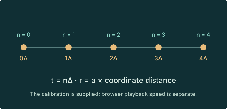
The record index n answers which completed state came before which other state. It does not, on its own, say how many seconds elapsed. To report duration we introduce a calibration Δ, the duration assigned to one outer update. A physical clock would require a reproducible process and an experimentally established relation between its readings and this index. [B03]
Likewise, the coordinate spacing in our graph is one mathematical unit. A length calibration a converts that spacing into an assigned physical length. The two scales are independent inputs in this exercise. Changing them changes the units reported, while the dimensionless state sequence remains exactly the same.
Motion in a completed-record account concerns relations between successive available configurations. It should not be confused with the traversal used to compute the configuration. Our central seed spreads symmetrically: its centre of weight stays at the origin even though the distribution changes. A widening distribution is therefore not the trajectory of a single moving particle. [B04]
Calibrate the same sequence
Step through completed updates and adjust the illustrative length and duration scales. The graph always follows the same μ = 0.1 rule. The readout gives the assigned elapsed time, root-mean-square distance from the origin, and the one-edge-per-update propagation bound.
Explore · teaching model v1
Teal: generated values. Gold: highlighted readout or reference.
Enable JavaScript to explore this model. The figure, worked values, and equations explain the same construction.
The units are examples, not fitted constants. A larger a increases all reported lengths; a larger Δ increases the reported elapsed time and reduces the ratio a/Δ. The playback button controls how quickly the browser shows records and does not change either calibration.
Distances, durations, and a dependency bound
The RMS quantity is measured about the fixed origin. For the symmetric central seed, it is also the spread about the centre of weight. It should not be interpreted as a particle speed. At n = 0 it vanishes; after one update with μ = 0.1 it equals a√0.6.
Each update can carry dependency across at most one graph edge. A site at distance d from the seed has zero weight before update d. This follows by induction: a site can receive a nonzero contribution only from its previous value or one of its neighbours. At boundaries, fewer outgoing edges change the spreading pattern.
Why this is not yet relativity
A finite dependency cone is weaker than Lorentz symmetry. Our cubic graph selects preferred directions, the update chooses a common discrete record sequence, and the diffusion rule is not a relativistic field equation. Assigning a numerical value to a/Δ does not remove these features.
The wider reconstruction programme separately addresses calibrated temporal pairing, cones, physical clocks, and observer transformations. A physical model must recover the appropriate relations among them, including established limits and measured clock comparisons. Those obligations cannot be discharged by changing the labels on an animation. [P01] [B10]
Continue to persistence to examine what survives repeated renewal in this particular update rule. For the broader question of proper clocks and boosts, see Clocks & relativity.