
A finite measurement outcome set does not discretize its time parameter; a continuum limit and an observable quotient are distinct constructions with different proof obligations.
The preprint’s organizing idea
Reconciling Discreteness and Continuity as Complementary Spectral Projections of Complex-Time Geometry in the Single Monad Model is a public Preprints.org manuscript. Its abstract proposes a shared temporal framework for discrete formation and continuous observed evolution. This guide develops the interpretation through explicit examples rather than treating the abstract’s broader physical claims as established.
Four distinctions matter immediately: a discrete outcome set, a discrete operator spectrum, a countable basis, and a discrete update parameter. None is simply a synonym for the others.
Continuous phases with two possible energies
Take an orthonormal pair |0⟩, |1⟩ and Hamiltonian H with energies 0 and Δ>0. Starting from (|0⟩+|1⟩)/sqrt(2), continuous evolution produces ψ(t)=(|0⟩+e−iΔt/ℏ|1⟩)/sqrt(2). An energy measurement still returns only 0 or Δ.
A measurement in the plus/minus basis instead gives P+(t)=(1+cos(Δt/ℏ))/2. The same two-dimensional state space supports a continuously varying probability. The example shows why an outcome count cannot by itself decide whether the underlying temporal parameter is discrete.
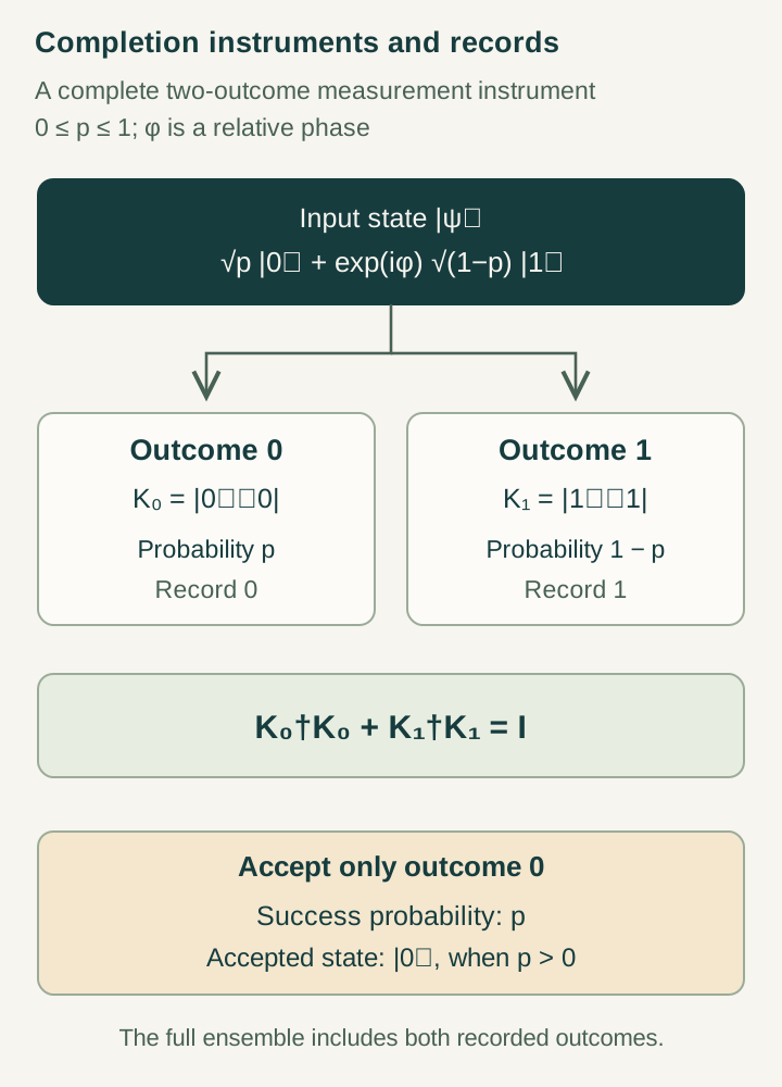
Open the full-size diagram →
Sampling creates another discrete object
Record that probability only at t=nτ. The observations now form a sequence indexed by integers, although the supplied state law remains continuous. Frequencies separated by 2π/τ produce the same sampled phase sequence. This is an exact aliasing ambiguity for that measurement schedule.
To identify a source frequency independently, one needs additional sampling intervals or other physical information. In DTT language, completed record order need not retain every detail of inner evolution. The observation protocol determines which distinctions survive.
A controlled route from lattice to derivative
For a smooth function, Taylor-expand f(x±a). The odd powers cancel in the centered second difference, leaving [f(x+a)−2f(x)+f(x−a)]/a²=f″(x)+(a²/12)f(4)(x)+higher terms under sufficient regularity.
This is a limit of a family indexed by a. A quotient instead identifies states that the selected tests cannot distinguish. A source construction can use both, but it should state whether the smooth law comes from shrinking lattice spacing, averaging over records, or a specific representation change. These routes have different error bounds and physical meanings.
A numerical comparison should therefore hold the measured interval fixed while refining a, then check that the discrepancy decreases at the claimed rate. Agreement at one spacing is a consistency example; convergence across a controlled family is a stronger result with a defined approximation error.
A projection must respect future experiments
If two alternatives carry a relative phase, their present path-insensitive label may be identical. A future recombination can distinguish them through interference. Erasing that phase in the reduced state would then lose predictive information.
SMM/DTT completion should therefore be defined against the admitted future procedures. A discrete public record can coexist with a richer continuous predictive state. The key source task is to derive when information is retained, when alternatives decohere, and why an observer can rely on the completed record across later interactions.
Connect the descriptions without conflating them
Read A209 with A82–A83 on future-test quotients and A111–A121 on explicit record formation. Use A153–A158 to distinguish spectral properties from metric information. Label each diagram arrow as a measurement, quotient, sampling map, or limit.
A concrete next question is whether one source model gives both an exact discrete instrument and a controlled smooth propagation law with an error estimate. If so, what observation scale makes the approximation valid, and which experiment detects its breakdown? This would turn the reconciliation into a quantitative relation between descriptions.
Continue with the articles
- Discrete and continuous spectral projections: a guide
Introduce the listed preprint’s proposal to relate discrete and continuous descriptions through projections. A future expansion should identify the precise objects on each side and their shared construction.
- When two histories count as the same observation
Introduce completion and observational equivalence as distinct ways of identifying histories. Explain why the tests available to an observer determine which differences survive.
- Test languages and observable quotients
Explore how richer tests alter the distinctions retained by a record model. Introduce the draft’s correspondence between test languages and observational congruences.
- A quantum source for generation and completion
Introduce the positive phase–dilation model as an explicit realization within quantum mechanics. Explain how it distinguishes inner work from completed observation without deriving quantum kinematics itself.
- A record that carries its own completion certificate
Introduce autonomous generation of a record and a flag certifying completion. Explain why the certificate must arise from the specified dynamics rather than an external declaration.
- From a continuous pointer to a binary memory
Explain the transfer of a Gaussian pointer response into a binary record with a generated flag. Discuss the threshold approximation and what controls its error.
- A spectral triple as a reconstruction interface
Introduce the algebra, Hilbert space, and Dirac-type operator used by the temporal spectral model. Explain the different jobs of observables, states, and spectral data.
Sources and reading
Read the original source for its exact formulation and edition. The examples on this page are explanatory reconstructions.