Quantum speed limits and the meaning of a cosmic refresh rate
A quantum system cannot pass between distinguishable states arbitrarily quickly at fixed dynamical resources. This supplies a quantitative test for language about inner ticks or cosmic refresh rates. A two-level calculation shows what a quantum speed limit constrains and why it does not by itself determine the speed of light.
A refresh rate counts something: distinguishable states, completed records, phase turns or elementary updates. These counts need not agree. A unitary system can accumulate phase without creating a new classical record, and an internal update can be invisible to every admitted receiver.
For SMM/DTT, the rate becomes physical when the model specifies what completion changes in an accessible state and how much energy, memory or control is needed. Quantum speed limits provide a benchmark at exactly this point. They connect a distinguishable change with the generator and the state’s available resources, rather than introducing a universal tick by definition. [1][2]
02The orthogonalization bound
For a pure state evolving under a time-independent Hamiltonian, the Mandelstam–Tamm bound limits the time to an orthogonal state by τ⊥ ≥ πℏ/(2ΔE), where ΔE is the energy standard deviation in the initial state. The bound concerns a particular state and generator. A small or vanishing energy spread can make orthogonalization slow or impossible.
This is not a universal time–energy operator commutator, nor a statement that a particle temporarily borrows energy. It is a dynamical distinguishability bound. Extensions to mixed states, open processes and controlled evolution require the appropriate distance and resource measure, so the simple expression should be used only in its stated setting. [2]
τ⊥ ≥ πℏ/(2ΔE)
Pure state, time-independent unitary evolution, orthogonal final state.
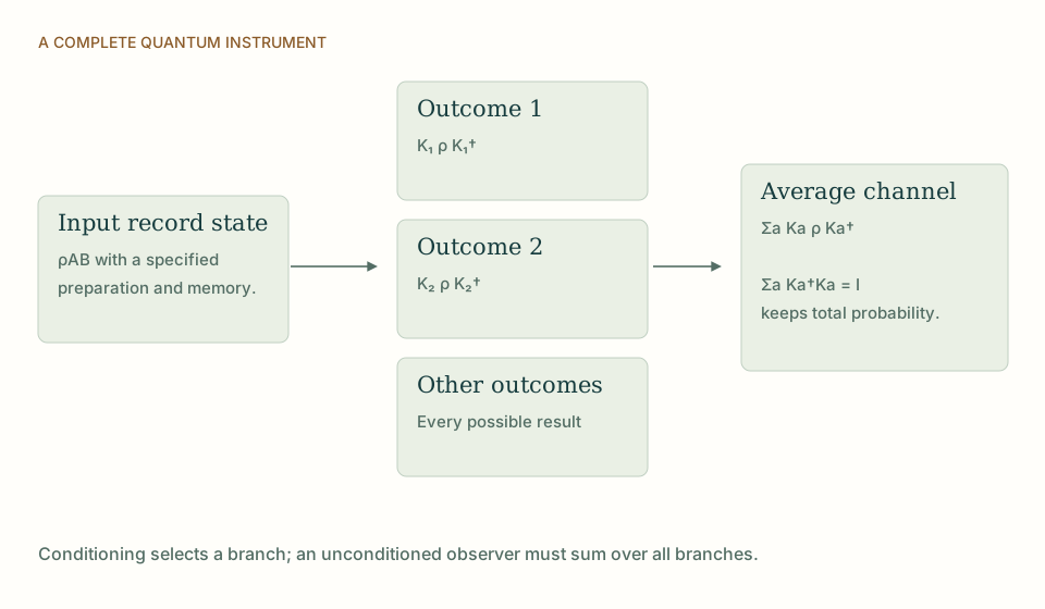
From a source process to a complete record instrument. Outcome probabilities, retained conditional states, and the outcome-averaged channel belong to the same instrument. Keeping every outcome prevents postselection from being mistaken for a signal. View full size ↗
03A two-level system that reaches the bound
Take H = (ℏΩ/2)σz and prepare the equal superposition |+⟩ of the two energy eigenstates. Its overlap with the initial state after time t is cos(Ωt/2), up to the conventional overall phase. The first zero occurs at t = π/Ω.
The energy spread is ΔE = ℏΩ/2. Substituting this in the bound gives πℏ/[2(ℏΩ/2)] = π/Ω, exactly the calculated orthogonalization time. The example shows how the clock-like rate depends on the supplied frequency Ω. It gives a complete benchmark while leaving the physical origin of that frequency open.
The angular frequency Ω is positive in this example.
04From internal change to recorded completion
An orthogonal state transition can support a perfectly distinguishable tick, but a persistent clock also needs a readout and memory. Repeatedly observing the system can alter its dynamics, and resetting it requires a physical protocol. The energy spread of the isolated two-level system is therefore not a complete resource budget for an indefinitely functioning clock.
A DTT completion instrument could use such transitions as part of its internal mechanism. The source model would then have to account for the clock’s preparation, repeated readout, correlations with retained records and stability under allowed operations. This is a constructive way to connect hidden generation to measured duration.
05Why this does not derive c
A frequency has units of inverse time. A propagation speed additionally requires a length per relevant transition and a definition of the signal whose influence is tracked. Multiplying a tick rate by a chosen spatial step produces a velocity, but the length, synchronization and common applicability to different species remain physical inputs.
Quantum speed limits also depend on the state’s energy resources. They are not automatically universal causal cones. A theory could combine a source-generated metric with an influence bound and a physical clock law, but the equality among those quantities must be shown. The common-source target is stronger than any one of these separate ingredients. [1]
06State change, a completed record and a usable tick
An evolving system can acquire a small phase without producing a distinguishable clock tick. For the two-level example, the return probability to the initial state changes continuously, and intermediate states need not be perfectly distinguishable from the initial preparation in one measurement. The orthogonalization bound answers a particular distinguishability question. A practical clock may operate with imperfect discrimination and quantify its tick error, resolution and disturbance instead.
A temporal source model therefore needs a completion criterion as well as a Hamiltonian. The receiver might announce a tick when a specified instrument registers a transition, when a phase estimate crosses a threshold, or when a stable record becomes available. Those procedures can have different timing statistics even for the same underlying evolution. Deriving their relationship to the six nested operations would connect a dynamical speed bound with an actual observation protocol. It would also expose which resources are required to make successive ticks reliable rather than simply label every internal change as a measured instant.
07A sharper use of the refresh picture
The language of refresh becomes useful when it predicts a resource-dependent bound on accessible record production. A model can calculate how many reliably distinguishable completions fit into a clock interval at fixed energy spread and memory capacity. It can then test whether a proposed inner architecture approaches or falls below the relevant limit.
Such a bound would be a real restriction on implementations of SMM/DTT even if it reproduced standard quantum mechanics. A further breakthrough would derive the physical action scale and common propagation law from the same source dynamics. The two-level benchmark keeps that larger ambition connected to a calculation whose assumptions and conclusion are fully visible.
THE SAME QUESTION, DIFFERENT STARTING POINTS
The comparison at a glance
Question
SMM/DTT
Mandelstam–Tamm bound
Refresh
Define a tick through an accessible completed change.
Quantum speed limits bound distinguishable state evolution.
Resource
Include generator, state, readout and retained memory.
The basic bound depends on the state’s energy spread.
Universal speed
Derive length and common signal propagation together with time.
A temporal orthogonalization bound alone does not fix c.
KEEP THE CONNECTION
Key ideas
The Mandelstam–Tamm bound concerns distinguishable state evolution at specified energy spread.
A two-level superposition saturates the bound at π/Ω.
A physical refresh interpretation still needs length, readout, memory and a common signal law.
References support the comparator and the specific mathematical or interpretive claims indicated. SMM/DTT connections are developed in the analysis above.