
Adjacency, metric and propagation are distinct outputs. A local completed circuit gives a graph support bound; a measured speed additionally needs length and clock calibration.
What you will learn
- Calculate weighted shortest-path distance.
- Explain why cubic adjacency does not automatically give Euclidean distance.
- Convert a local update bound into a conditional propagation-speed bound.
Before you begin: Lessons 01–04. You need addition, the triangle inequality and the distinction between a full state and its display.
Let operations define neighbours
Begin with completed record labels. Declare two labels adjacent when a permitted elementary comparison connects them. This produces a graph: labels are vertices and comparisons are edges. A drawing helps us see the graph, but positions on the page do not determine its operational geometry. Adding an edge between distant-looking labels makes them neighbours by definition of the permitted comparisons.
In an SMM construction, these edges should arise from the source's operation law and persistent memory. A programmed translation table can produce a regular lattice and establish possibility. Showing why that structure is selected and remains stable under allowed disturbances is a stronger physical result. Keep the preparation rule separate from the later dynamics acting on the prepared graph.
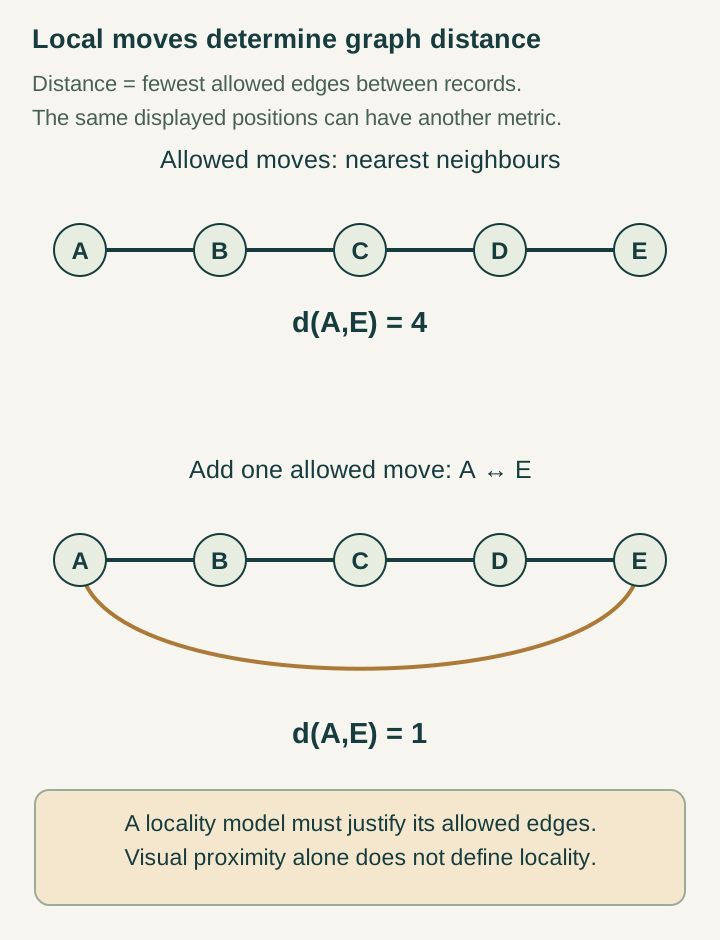
Open the full-size diagram →
Worked example: the cheaper route sets distance
Assign positive costs to edges and define distance as the least total cost of a connecting path. Suppose A–B costs two, B–C costs three and A–C costs seven. The direct route from A to C costs seven, while the route through B costs 2+3=5. The distance is therefore five.
This distance can also be read through constrained observables. Let f assign a real reading to each vertex, with differences no greater than an edge's cost. Along any path, the triangle inequality bounds the total reading difference by the path cost. The choice f(A)=0, f(B)=2, f(C)=5 satisfies all three constraints and attains five. Local comparison limits have therefore reconstructed the same global distance.
Three directions do not choose one metric
Consider a square lattice with unit horizontal and vertical edges. From (0,0) to (1,1), every allowed shortest route has two steps, so graph distance is two. A Euclidean ruler laid across the drawing gives √2. These answers measure different permitted comparisons. Simply making axial edges finer preserves the same preference for axial travel unless the comparison procedure also changes.
Likewise, a three-dimensional cubic graph has a Manhattan distance equal to the sum of absolute coordinate differences. Its number of sites in a large region can grow like a radius cubed, while its norm remains different from Euclidean length. Rank, growth dimension and metric answer different questions. An isotropic physical limit needs a justified additional mechanism rather than a relabelling of one diagnostic.
A finite law that preserves local influence
Put a register at each vertex. Suppose one completed episode first acts within individual sites and then exchanges dedicated ports across neighbouring edges. Assume the edge layer consists of disjoint port exchanges and that no unlisted controller channel connects distant sites. An initially local disturbance can affect only its original site and adjacent sites during that episode.
Repeat the argument: after k episodes its influence is contained in the graph neighbourhood of radius k. This is an induction. The first episode gives the one-step claim; each later episode adds at most one edge to every possible influence path. The result is an exact causal support bound for this circuit architecture. It does not require pretending that an internal counter scan is itself particle motion.
Add a ruler and an actual clock
Let each edge have calibrated length ℓ and let every completed episode take duration Δt measured by a specified clock. The preceding support bound becomes a maximum slope ℓ/Δt. For ℓ=3 length units and Δt=2 time units, four episodes take eight time units and reach at most twelve length units, giving slope 3/2.
A serial source may perform many internal operations to execute one episode, so assigning it the name tick does not establish Δt. Also inspect retained controller memory. A register that carries unknown information between distant sites creates a transport channel; its journey must be represented in the graph or excluded by the dynamics. Otherwise the claimed locality bound omits an actual route of influence.
Use separate tests before connecting the outputs
A practical geometry test first reconstructs adjacency from operations, then measures comparison lengths, then perturbs a local register and tracks accessible responses. Repeat after small changes to the source preparation. A robust construction should preserve its intended neighbourhoods and propagation rules together, with stated errors.
DTT makes the completion boundary especially important: the completed episode is where the retained graph and support statement are assessed. Six nested inner roles may organize the preparation, while the outer interface certifies the result. The locality guide develops the exact support proof and the metric guide develops normalized comparisons. Lesson 06 turns to another needed structure: a phase carrier supporting coherent dynamics before registration.
Try the exercises
Work through each question, then open the answer to compare the steps.
Exercise 1
If the direct A–C edge is changed from seven to four, calculate d(A,C) and exhibit a permitted reading f that attains it.
Show the worked answer
The indirect path still costs 2+3=5, while the direct path now costs four, so d(A,C)=4. Choose f(A)=0, f(B)=2 and f(C)=4. The three differences are two, two and four, bounded by edge costs two, three and four. This reading attains the new distance and verifies that the shortcut changes the operational metric.
Exercise 2
A disturbance is five edges from a detector. One episode permits one edge of influence, takes three clock units and each edge is two length units. Find the earliest allowed arrival and maximum slope.
Show the worked answer
Fewer than five episodes cannot connect the disturbance to the detector under the declared support bound. The earliest permitted time is therefore 5×3=15 clock units, over graph length 5×2=10. The maximum slope is 10/15=2/3 length units per clock unit. This is a lower bound on arrival time, not a guarantee that any signal actually reaches the detector at that time.
Continue with the articles
- Why local geometry can be statistically rare
Explain the entropy barrier to lattice-like relational memories in the stated permutation ensemble. The result concerns a specified preparation problem, not every possible mechanism for emergent space.
- Generating a neighborhood and preserving local transport
Separate reconstruction of spatial adjacency from the requirement that subsequent dynamics remain local. Explain the guarded transport rules used to preserve the generated metric.
- A finite-update cone
Introduce the bound relating horizontal displacement to temporal projection in the limiting-speed draft. Explain that the finite-update inequality is a stated geometric assumption.
- Graph distance from a normalized spectral block
Introduce the graph-block construction whose Connes distance equals weighted shortest-path distance. Explain the normalization assumptions behind that equality.