
The supplied signed pairing gives ranks 1,1,2,2,3,3 and maps 64 binary addresses to 27 sites. Uniform source sampling gives unequal site weights.
What you will learn
- Derive the paired-readout rank sequence.
- Calculate binary site multiplicities and probabilities.
- Distinguish an internal scan from physical motion and a spatial image from predictive memory.
Before you begin: Lessons 01–03. A vector direction means an independently variable coordinate; no prior linear algebra is required.
Supply a frame and define the readout
Choose three independent directions e1, e2, e3 and a positive length ℓ. Independent means no direction can be formed by combining the other two. Use the six counter digits introduced in Lesson 02 and define a spatial candidate by pairing adjacent digits with opposite signs.
This rule deliberately supplies a frame, a scale and a pairing. It gives a concrete question we can solve: what information appears in Q as nested digits become available? Showing the answer is exact for this construction is stronger than an analogy, while deriving why the source selects this particular construction remains another task.
Why the rank rises every second role
The rank here counts independent directions in the set of available outputs. When only d1 varies, every output lies along e1. Allowing d2 adds negative contributions along that same direction. It changes available positions, but cannot add a second direction. The third digit introduces e2; its partner again adds no new direction.
Repeating the argument for the final pair gives ranks 1,1,2,2,3,3. Each newly claimed direction actually occurs by setting its first digit to one and the others to zero, so these are attained ranks rather than upper bounds. The result does not say that any imaginable six-stage process yields three-dimensional space. Its signed columns and independent frame do the mathematical work.
Worked example: count one pair first
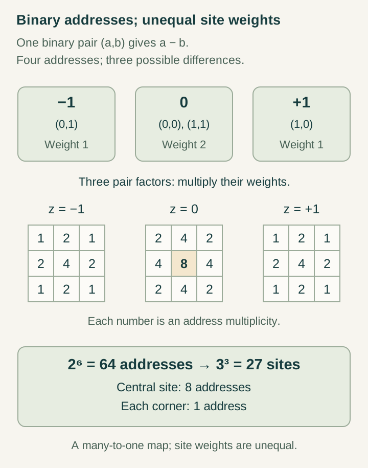
For binary digits, one pair has four possibilities. The pairs (0,0) and (1,1) both give difference zero, while (1,0) gives +1 and (0,1) gives −1. Therefore the values −1,0,+1 have multiplicities 1,2,1. Under uniform preparation of the four pair states, their probabilities are 1/4,1/2,1/4.
Three independent pairs give 4³=64 addresses and 3³=27 coordinate triples. Multiplicities multiply: the origin has 2×2×2=8 representatives, a site such as (1,0,0) has four, and (1,1,1) has one. Their probabilities are respectively 1/8, 1/16 and 1/64. The drawing is regularly spaced, but the declared sampling measure is visibly nonuniform.
Open the full-size diagram →
Check the entire distribution
Group the sites by the number j of nonzero coordinates. There is one central site, six sites with one nonzero coordinate, twelve with two and eight with three. Their multiplicities are eight, four, two and one respectively. The site count is 1+6+12+8=27 and the address count is 8+24+24+8=64.
This gives a useful independent normalization check: the four class probabilities are 1/8,3/8,3/8,1/8 and sum to one. To sample sites uniformly would require a different preparation or weighting rule. For example, each address at site y could receive probability 1/[27M(y)], where M(y) is that site's multiplicity. Summing its M(y) contributions then gives exactly 1/27.
The spatial display forgets a carry
Use the binary-spatial-readout demonstration at addresses zero and three. Their least-significant-first digit strings are 000000 and 110000. Both give Q=0. Increment each address once. Address one gives ℓe1, whereas address four gives ℓe2.
This is Lesson 03's failed-autonomy test in a spatial setting. An observer who retained only the current site could not know which successor to choose. Keeping the carry information repairs the prediction. The example also cautions against interpreting the counter's ordered scan as a particle trajectory: a carry can create a projected jump. A law of local motion on the retained sites must be specified and tested separately.
What three coordinates have established
We have an exact finite image with three independent directions, calculated multiplicities and a known loss of predictive information. We do not yet have a physical distance rule, an experimentally calibrated ruler or a bound on signal propagation. Even orthogonality was not required for the rank calculation; assigning Euclidean lengths would add a metric to the independent frame.
The deeper paired-rank derivation proves a six-channel lower bound under an opposite-pair architecture and explains alternatives outside those assumptions. The next lesson instead takes the generated-record perspective forward: choose which records are adjacent, derive distances from permitted comparisons, and determine whether the actual dynamics respects those relations.
Try the exercises
Work through each question, then open the answer to compare the steps.
Exercise 1
For the binary site (−1,0,1), find its multiplicity and probability under uniform address sampling.
Show the worked answer
The first coordinate has one representative, the second has two, and the third has one. Independence gives M=1×2×1=2. Since each of the 64 addresses has probability 1/64, the site's probability is 2/64=1/32. It belongs to the class with two nonzero coordinates; there are twelve such sites, together carrying probability 12/32=3/8.
Exercise 2
At radix three, each digit is 0, 1 or 2. List the multiplicities of one difference and find the final site count and origin probability.
Show the worked answer
The differences −2,−1,0,1,2 have respectively 1,2,3,2,1 representatives. The total is nine, as required for two ternary digits. Three pairs therefore give 5³=125 sites from 3⁶=729 addresses. The origin has 3³=27 representatives, so its probability is 27/729=1/27 under uniform address sampling. The rank remains three.
Continue with the articles
- Six inner stages and one publication interface
Explain the hierarchy of readout ranks 1, 1, 2, 2, 3, 3 followed by completion. These are nested functional roles rather than six independently readable temporal coordinates.
- Generating a neighborhood and preserving local transport
Separate reconstruction of spatial adjacency from the requirement that subsequent dynamics remain local. Explain the guarded transport rules used to preserve the generated metric.
- What spatial readout forgets
Investigate information lost when a full generative state is reduced to spatial records. Explain why an apparently complete geometry may still be insufficient for autonomous prediction.