Quantum phase and complex structure: SMM/DTT and standard Hilbert-space quantum mechanics

01The question behind this comparison

Quantum phase is a relation among amplitudes that becomes observable when alternatives recombine. An overall phase multiplies all amplitudes equally and does not change ordinary measurement probabilities; a relative phase can change them sharply. The relevant scalar unit in standard quantum mechanics obeys i²=−1. A split-complex unit j with j²=+1 describes a different algebra and cannot simply replace i while preserving the usual positive probability rule.

The DTT programme can connect temporal organization to phase by asking whether real source dynamics selects a compatible complex structure. Such a selection is a mathematical statement about an operator and the symmetries that commute with it. It is more specific than calling one temporal role imaginary. Establishing a complex structure does not yet establish the Hamiltonian, the Born rule or the physical meaning of its phase scale. ^{[2] [3]}

02The SMM/DTT starting point

The Single Monad Model begins with one nonspatial generative source. The Duality of Time Theory distinguishes the source’s inner production from the outer order in which completed records become accessible. Its six inner levels are nested functional roles of one process: a higher role organizes lower-level work. The seventh is the completion or observation interface. They are neither six independent clocks nor six additional time coordinates.

This distinction supplies a useful research question: which features of an observed world can follow from the way a source produces, retains and releases information? A concrete answer needs a state space, an autonomous update, retained memory and a rule connecting completion to an accessible measurement. In the constructions discussed here, those mathematical ingredients are stated explicitly. A successful finite example establishes what its specified mechanism can do; further arguments connect it to physical particles, spacetime or universal laws. ^[1]

03How the comparator works

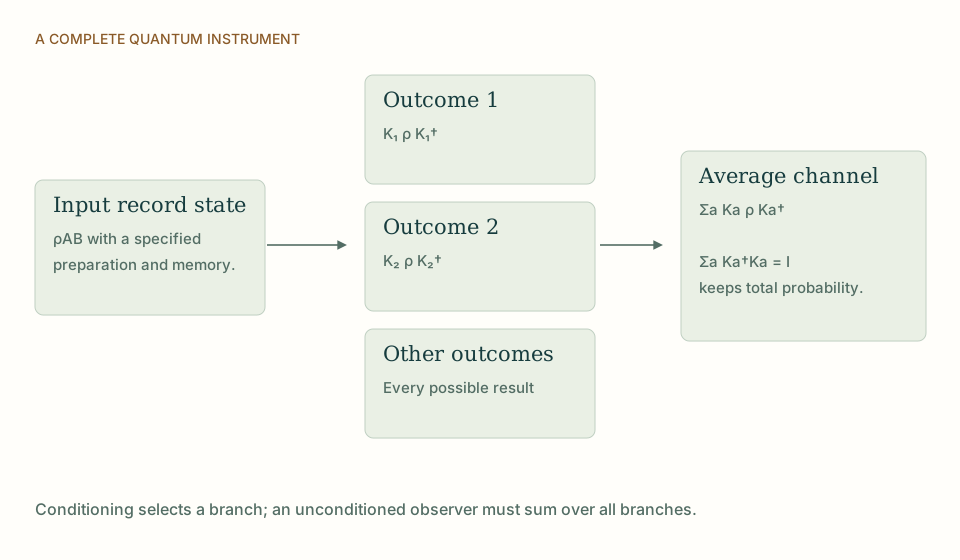
Operational quantum mechanics represents a preparation by a positive density operator of unit trace. A measurement outcome corresponds to an effect, and an instrument specifies both its probability and the conditional state left behind. Closed evolution is unitary; an open system can evolve by a completely positive, trace-preserving map. These ingredients are sufficient to calculate laboratory statistics without deciding whether the wavefunction describes an ontic object, a relation or an agent’s expectations.

The instrument language is especially close to DTT’s distinction between production and accessible records. An unobserved interaction and a registered outcome are mathematically different objects. Yet an ordinary instrument does not itself contain a hidden generative time, nor does a sequence of instruments derive the space in which laboratories operate. It provides a precise interface against which a proposed inner process can be tested: if the process reproduces exactly the same instruments, the difference is explanatory or structural unless another accessible measurement distinguishes it. ^[2]

04The decisive comparison

Hilbert-space quantum mechanics assumes an ordinary complex structure in its conventional formulation. DTT can ask a deeper reconstruction question: under what conditions does real source dynamics select the operator J that makes the state space effectively complex? This is a mathematically meaningful task because J²=−I is an exact condition, and its compatibility with a dynamical generator can be tested without appealing to metaphorical imaginary motion.

The distinction is especially important when split-complex time is also used. Hyperbolic kinematics may organize an indefinite causal form, while ordinary phase rotations preserve the positive structure used in quantum probabilities. The two operations have different generators and cannot be interchanged by notation. A successful DTT interface could relate them through a readout or spectral decomposition, thereby explaining why different aspects of the observed theory use different geometric structures. Yet selecting J alone leaves the physical action scale and Hamiltonian unspecified. The constructive result should therefore identify exactly which freedom has been removed: the existence or uniqueness of a compatible phase, rather than the entire content of quantum dynamics. ^{[2] [3]}

05Worked benchmark

On a real two-dimensional space take J=[[0,−1],[1,0]]. Direct multiplication gives J²=−I. The exponential of θJ is cosθ I+sinθ J, a rotation that preserves x²+y². Identifying (x,y) with z=x+iy converts that same real evolution into z↦e^{iθ}z. No second physical time coordinate was introduced.

By contrast, K=[[0,1],[1,0]] obeys K²=I. Its exponential is coshη I+sinhη K and preserves x²−y². This hyperbolic transformation is appropriate for an indefinite quadratic form, not the Euclidean norm that supplies an ordinary one-component Born probability. A temporal reconstruction may use both structures in different roles, but it needs a map explaining how they coexist. Substituting η=iθ is an analytic continuation of formulas; it is not a demonstration that a physical process rotates one type of time into the other. ^{[2] [3]}

06What follows for the source programme

This comparison turns a suggestive dual-time vocabulary into a testable algebraic question: what physical constraints select J, and which transformations preserve that selection? If several inequivalent complex structures remain allowed, further dynamics or boundary conditions are needed. A rank-three quaternionic readout can organize rotations and phase actions, but its algebraic rank must not be mistaken for a proof of an emergent three-dimensional metric manifold. ^{[2] [3]}

THE SAME QUESTION, DIFFERENT STARTING POINTS

The comparison at a glance

Continue on SMONAD

• Split-complex time and ordinary quantum phase →

  Connects this comparison with the author’s underlying construction.

• Selecting phase by polar decomposition →

  Connects this comparison with the author’s underlying construction.

• Completion, commutants, and positive frequency →

  Connects this comparison with the author’s underlying construction.

• Real-commutant phase selection: a paper guide →

  Connects this comparison with the author’s underlying construction.

• SMM/DTT research claim map: results, assumptions and open targets →

  Places the comparison alongside the programme’s published results, assumptions and open targets.