
A reserved observable is a unique calibrated prediction only when it is constant across all admissible models matching the calibration. A discriminating test then compares that consequence with a specified alternative and its uncertainties.
Freeze the equations as well as the parameter values
Record the source update, admissible states, completion instrument, physical dictionary and approximation order. List all data used to choose numbers or functional forms, including indirect input through fitted constants. Separate those calibration observations from reserved comparisons before evaluating the latter. Selecting among many operators after seeing the entire residual pattern consumes test information even if the final operator has only one coefficient.
This is especially important for SMM/DTT’s common-source claim. A structural receiver, action standard and clock interface may each be supplied or calibrated at the current stage. A conditional prediction can still be valuable, provided those dependencies are visible. Reconstructing a coupling used to fix response normalization is a consistency check; the next unchanged model output is the candidate prediction.
Check the full family left by the calibration
Let p denote model parameters, C(p) the calibrated observable and Ψ(p) a reserved quantity. Calibration selects all admissible p satisfying C(p)=Cobs. A unique output requires Ψ to have the same value everywhere in this family. Otherwise report the allowed range or add an independent calibration.
For an exact toy example, let x,y>0 and calibrate x+y=1. The proposed output Ψ=x−y ranges over (−1,1), so the calibration does not predict it. By contrast, Φ=2(x+y) is fixed at two throughout the family. A second input x=1/4 gives y=3/4 and Ψ=−1/2. That second observable has removed the ambiguity; it cannot simultaneously be counted as an independently predicted result.
Use local derivatives without confusing them with a proof
At a regular point, parameter variations preserving calibration to first order lie in ker dC. If dΨ is nonzero on one such direction, the reserved quantity is locally ambiguous. If dΨ vanishes on all such directions throughout a connected smooth calibration family, integration along paths establishes constancy there.
Checking only one point is insufficient: Ψ(x)=x² has zero derivative at zero but varies nearby. Disconnected branches and discrete choices such as receiver grammar need separate checks. In a noisy calculation, inspect the singular values of the covariance-weighted sensitivity matrix. A small singular value signals an unstable inference even when exact rank is formally sufficient. The clock-selection guide supplies a concrete example where two almost parallel readouts have this problem.
Calculate a shared spectral consequence before fitting its amplitude
Use h=2πa to convert energy to ordinary frequency. Take the explicitly illustrative first-order contact level shift δEnS=K/n³. The signed transition shifts are hδν12=K(1/8−1)=−7K/8 and hδν23=K(1/27−1/8)=−19K/216. Therefore a single amplitude predicts:
Calibrating K on the first line leaves the second as a conditional test. A third stationary transition must also respect δν13=δν12+δν23; it is not another free offset. For q connected levels there are q−1 independent stationary energy differences. Extra measured edges can check consistency and reduce uncertainty without creating new independent level parameters. A contact pattern remains a comparison example until a source model derives its operator and coefficient.
Ask whether conventional uncertainty can produce the same pattern
Write a residual vector as r=Sc+Nη+ε, with source-shape columns S, conventional nuisance columns N and covariance Σ. If a source column lies in the nuisance span over the selected channels, those data cannot separate the mechanisms without independent constraints. Counting named coefficients is less useful than counting independent directions after calibration and exact transition identities are handled.
For the two-line contact check, set k=19/189 and D=r23−kr12. If both residuals have variance σ² and correlation ρ, then Var(D)=σ²(1+k²−2kρ). The subtraction may cancel a shared uncertainty but still retain independent noise. Freeze weights and covariance conventions before examining reserved data, and keep numerical solver error separate from uncertainty in physical inputs.
Connect the predicted relation to the source architecture
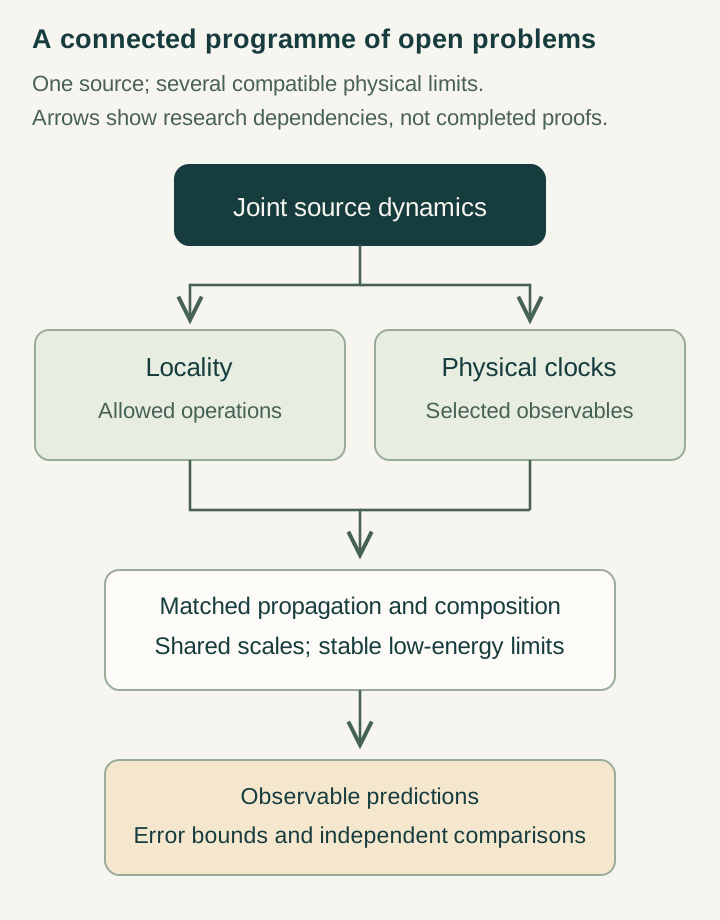
A meaningful SMM/DTT advance would derive a relation among independently defined coefficients from one autonomous update. Six nested inner dependencies should constrain how records, clocks and response are produced; the outer completion rule should expose their joint statistics. Naming every module as part of one source does not itself impose those relations.
Open the full-size diagram →
This conceptual diagram marks the successive obligations. Compare the candidate with an ordinary quantum or atomic model implementing the same accessible operations and permitted memory. A difference becomes distinctive only relative to that declared class. A record-only model can fail while a larger one-time hidden-state comparator succeeds; excluding the former does not exclude the latter.
State what success, failure and revision would mean
Specify the reserved observables, predicted interval or distribution, covariance treatment and decision criterion. An agreement supports the restricted relation under those assumptions; a disagreement can challenge the source operator, normalization, matching or baseline. Preserve the original prediction while diagnosing which component failed. A revised operator should receive a fresh validation set rather than retrospectively absorbing every discrepancy.
The immediate deliverable is a reproducible mathematical comparison with no fabricated measurements. It can identify an exact new relation, a surviving free direction or an informative bound. That is how a broad source interpretation becomes a sequence of assessable claims. The consistency guide checks the model before this stage, and the claims guide distinguishes conditional constructions from completed physical derivations.
A null result has a useful scope too: it bounds the specified coefficient within the tested channels and sensitivity. It need not reject every source interpretation. Report that bounded claim directly, including any degeneracy with conventional operators that prevents a separate coefficient limit.
Continue with the articles
- Identifiability: can observations determine the model?
Explain why a collection of observable constants can leave parameter directions unresolved. Use the draft’s two remaining directions to distinguish a good fit from unique reconstruction.
- Prediction after calibration
Present the calibration-fiber criterion for a conditional prediction. An additional observable must be fixed across the allowed calibrated models to avoid merely reusing its target value.
- Freeze parameters before predicting spectroscopy
Explain the post-freeze strategy proposed for atomic observables. A spectroscopy comparison becomes informative when its coefficients are fixed without using the same transitions as targets.
- Recovering a QED baseline before adding residuals
A proposed methodology article for the fine-structure program. Explain how agreement with a standard baseline must be established before a residual can be attributed to new temporal dynamics.
- What would count as a DTT spectroscopic residual?
Outline criteria for a meaningful residual: a specified model, fixed coefficients, uncertainty control, and a pattern across observables. The skeleton draft motivates this task but does not complete it.
- Differential spectroscopy as a test strategy
Explain why differences between transitions can test a shared model more strongly than a single fitted line. Develop the proposed holonomy comparison as an overconstrained protocol.
- Designing an overconstrained atomic test
Turn the skeleton draft’s research direction into a practical analysis plan. Require more independent observables than fitted parameters and predeclare the cross-state prediction rules.
- How a protocol can reveal dual-time structure
Outline ways to move beyond the finite prepared linear interface: protocol-dependent access, noncommuting transport, or richer memory. Each route must be defined as an observable procedure.