

Neutrality is a starting condition, not a bound state
Two opposite charges can form a neutral pair, but neutrality alone does not show that the pair remains together. Binding means that a specified Hamiltonian supports a normalizable state below the energy of separated constituents. A proposed source model must supply the attraction and the competing kinetic response.
The laboratory starts with the conventional nonrelativistic relative-coordinate Hamiltonian H=p²/(2μ)−κ/r, where μ is the reduced mass and κ>0 is the attractive Coulomb coefficient. Space is three-dimensional, the probability rule is quantum mechanical, and the dissociation threshold is zero. These are explicit inputs.
For the SMM/DTT programme, this provides a concrete target: a common generation law should fix the kinetic and mediator responses together. Giving an interaction a geometrical interpretation does not yet choose its normalization or prove binding. The source's comparison rule and dynamical coefficients must cooperate. [M06] [M07] [B16]
Squeeze and spread the same normalized state
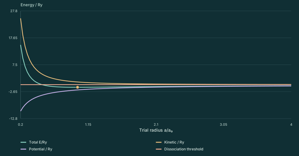
The scale slider changes the radius a of a normalized exponential trial state. The graph separates kinetic, potential, and total energy. Small a squeezes the state and raises its momentum spread. Large a spreads it out and weakens the attraction.
Interactive calculation
Play scans Trial radius a/a₀. Step advances it. No animation starts automatically.
Enable JavaScript for adjustable values. The static figure and worked calculation remain available.
At s=a/aB=1, the scaled kinetic energy is +1, the potential energy is −2, and the total is −1. At s=1/2 the two terms are +4 and −4, giving zero total energy. At s=2 they are +1/4 and −1, giving −3/4. The optimum is neither collapse nor unlimited spreading.
The curve represents expectation values in a family of quantum states. It is not the potential energy of a classical electron orbit. The optimum radius characterizes a distribution; it does not assign every detection the same distance.
Find the minimum and check its meaning
Normalization follows by integrating 4πr²|ψ|² over r≥0. For this family, ⟨1/r⟩=1/a and the gradient norm gives ⟨p²⟩=ℏ²/a². Substitution yields the energy curve without a trajectory assumption.
The derivative vanishes only at s=1, and the square identity proves that this is the unique minimum in the trial family. Here the result is stronger than a generic variational estimate: the minimizing exponential is also an exact eigenfunction of the supplied Coulomb operator.
A global check comes from completing a square in the quadratic form. With D=ℏ²/(2μ) and aB=2D/κ, the energy plus D/aB² equals D∫|∇ψ+r̂ψ/aB|²d³r for normalized admissible states. The nonnegative right side supplies the lower bound, and the exponential saturates it. The three-dimensional identity ∇·r̂=2/r is the geometric step behind this calculation.
The second derivative at the optimum is positive, so a small size error raises the energy to quadratic order. This is a local stability check within the exponential family. Stability against other deformations follows from the stronger lower-bound identity, rather than from the plotted curve alone.
One scale must explain several outputs
The derived radius and binding energy use the same μ, κ, and ℏ. Fitting the radius with one normalization and the energy with another would break the declared model. This shared dependence is precisely the kind of cross-check sought in a common-source reconstruction. [M08] [M09]
The calculation does not select the physical value of κ. Every positive κ has a corresponding bound state in this model. It also does not include relativity, radiation, spin-dependent interactions, or nuclear structure. Those effects require an extended operator and a controlled regime of approximation. The finite-size minimum remains a useful benchmark against which a proposed microscopic reduction can be checked.
The original interaction-and-binding guide addresses how an effective attraction can arise. The complete hydrogen guide gives the atomic benchmark. Continue to the radial distribution to see what the finite scale predicts for observations.