


Persistence is a property of a record
In the Single Monad picture, a material object is a reproducible organization generated through time. The mathematical question is what makes that organization survive the next completed update. An answer must identify both the state that evolves and the measurements that recognize the pattern. A repeated name or a drawing of a loop is not yet a stability law. [M01] [M02]
A useful first example is an eigenmode of a unitary update U. If Uψ=e−iωψ, repeated updates change only an overall phase. Every expectation ψ†Aψ of a fixed observable A remains unchanged. Internal phase evolution and a stationary measured pattern can therefore coexist exactly.
The same idea becomes richer when two modes are combined. Their individual densities can remain stationary while their relative phase changes an interference term. Persistence then means a predictable recurring structure, not necessarily a density that is fixed at every point. The laboratory separates these two possibilities on a mathematical circle.
Move between one mode and a coherent pair
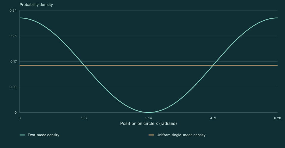
The ring coordinate x runs from 0 to 2π. A weight p sets the first mode's population, and the phase φ sets its comparison with a second mode having one angular winding. Play advances φ; the peak moves around the ring. This animation shows an exact probability density, not a simulated particle trajectory.
Interactive calculation
Play scans Relative phase φ (degrees). Step advances it. No animation starts automatically.
Enable JavaScript for adjustable values. The static figure and worked calculation remain available.
At p=1 or p=0, only one mode remains and the density is uniform. At p=1/2 the contrast is maximal. Set φ=0: the density is largest at x=0 and vanishes at x=π. Set φ=π: the bright and dark positions exchange. A full 2π phase cycle restores the same distribution.
At p=0.8 the contrast is 2√(0.8×0.2)=0.8. The maximum and minimum densities are respectively 1.8/(2π) and 0.2/(2π). The area under the entire curve remains one as the contrast and peak position change.
Calculate the retained pattern
Orthogonality removes the integrated cross term, so the state is normalized for every 0≤p≤1. Taking the squared modulus gives the plotted density:
Its integral is one because the cosine integrates to zero over a full circle. Its minimum is nonnegative because 2√(p(1−p))≤1. These checks distinguish a legitimate probability model from an arbitrary moving wave.
If the two eigenfrequencies are ω₀ and ω₁, the evolving relative angle is φ=(ω₁−ω₀)T plus its initial value. A common shift of both frequencies adds an overall state phase and leaves ρ unchanged. For a nonzero difference, the probability pattern repeats after 2π/|ω₁−ω₀|. Turning that parameter into a measured duration requires a physical clock.
A useful comparison is to average the density over the entire ring before and after a phase change. Both averages agree, while small local bins can differ. This demonstrates how one measurement can erase a distinction that another admissible measurement retains.
From a recurrent mode to matter
The example supplies a state space, a two-mode carrier, and a probability rule. It does not supply charge, particle statistics, interactions, or three-dimensional localization. A material identification requires those compatible properties to follow from the same dynamics. The published reconstruction and phase-selection results motivate parts of that dependency chain; they should not be read as an atomic spectrum derived by this ring experiment. [P01] [P03] [B16]
For SMM/DTT, the next constructive step is a retained carrier that is stable under inner operations and supports reproducible outer tests. Stability should be checked against specified disturbances, not assumed from recurrence alone. A pattern may recur perfectly in isolation and be rapidly destroyed by a coupling to its environment.
Continue to dispersion to connect a mode's phase advance to propagation. The original persistent-excitations guide develops eigenstates and a coupled two-state stability example. Observation explains why the selected readout matters.