
A local unitary walk provides an exact finite propagation bound and a calculable group velocity. Its shared physical interpretation as c depends on a common completion duration and on matching the propagation laws of other sectors.
Three quantities that should be distinguished
A circuit bound states how far the support of a disturbance can spread per completed update. A group velocity describes the motion of a sufficiently narrow wave packet through a chosen dispersion band. A causal or signal front concerns the earliest controllable influence. These quantities can agree in a particular regime, but their equality is a result, not a definition.
SMM/DTT seeks a common generative explanation of these structures. The inner process builds and updates a configuration; outer records supply the measured duration. A useful model must identify which source operations actually carry information between completed locations before interpreting their rate as a physical speed.
A finite update gives an exact support statement
Consider a lattice whose completed update combines an on-site operation with a shift by at most one edge. After one update, a local observable can involve only its original sites and their neighbours. Repeating this argument shows that k updates enlarge its support by at most k graph steps.
If each edge has length ℓ and every episode has physical duration Δt, the corresponding slope is ℓ/Δt. The proof excludes additional long-range couplings or a mobile hidden memory bus. A source that mediates remote influence through an unaccounted register would require that register's interactions to be included in the bound.
A local matter mode with exact dispersion
Take a two-component carrier, rotate it through C=exp(−iθσx) and shift its components in opposite directions. In a dimensionless momentum variable k, the shift is S(k)=exp(−ikσz). The completed unitary U(k)=S(k)C has eigenvalues exp(±iω).
The trace of U is twice cos θ cos k, which proves the relation. This is a concrete matter model on a supplied lattice. It connects internal mixing and spatial transfer within one update, illustrating the kind of output a more fundamental six-level generative construction would need to select.
Deriving the band-speed bound
Differentiate the cosine relation on a smooth eigenphase branch. The group speed in physical units is (ℓ/Δt)dω/dk. A short identity controls it:
sin²ω−cos²θ sin²k=sin²θ≥0.
Therefore |vg|≤ℓ/Δt.
For θ=π/3 and k=π/2, the selected branch has ω=π/2 and dω/dk=1/2. The packet speed is exactly half the update-bound slope. A band can therefore propagate more slowly than the fastest support allowed by the same local operation. The support theorem and the derivative calculation establish different parts of the transport description.
Why massive waves need not move at the boundary
For a relativistic positive-energy band E(p)=√(m²c⁴+c²p²), differentiation gives the group velocity v=c²p/E. For nonzero mass and finite momentum, |v|<c. The associated phase velocity E/p can exceed c, but it does not describe the speed of a localized controllable disturbance.
The distinction matters when a temporal model assigns a recurrence frequency to a particle. A large phase frequency does not imply a large signal speed. The propagation law comes from how that frequency changes with momentum, together with the locality of the full update. Rest recurrence and spatial transport must be calibrated against the same completed clock.
What makes the speed common to different fields?
A geometry permits many equations. A scalar field with highest-derivative part ∂²tφ−v²∇²φ has characteristic speed v; choosing v independently of the electromagnetic coefficient gives another cone. Merely placing both equations on one record archive does not force their coefficients to coincide.
A common-source derivation should obtain compatible highest-derivative propagation terms from one interaction law and independently fixed normalization. Masses and lower-order potentials can then differ while the characteristic cone remains common. This is the precise content behind the SMM intuition that distinct matter patterns share a generative origin.
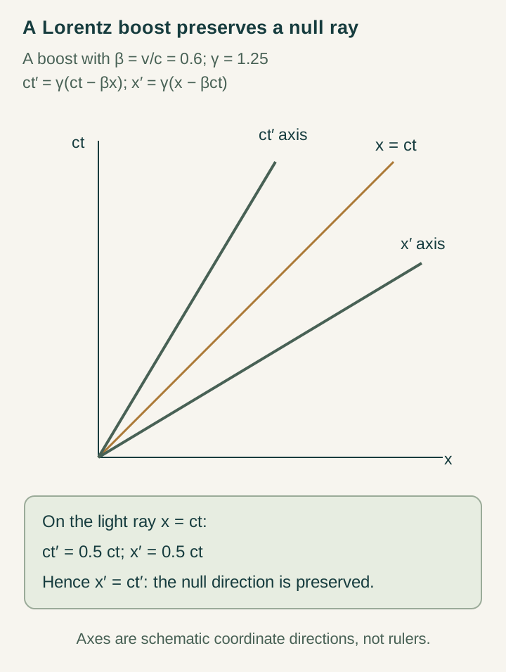
Open the full-size diagram →
A numerical value is partly a unit statement
Rescale the numerical length coordinate by a positive factor a and the clock coordinate by b. Every represented speed changes by a/b. Thus a derivation of a common invariant speed and a derivation of its numeral in chosen units are different tasks.
Dimensionless comparisons survive this freedom. Two independently calibrated matter sectors with different ratios to the same clock-defined c reveal a physical disagreement. Conversely, redistributing a factor between an inner activity scale and its outer clock conversion without changing their product is not a new prediction.
The next DTT calculation
Generate a local archive, a material clock and at least two propagating carriers from one declared autonomous update. Include the retained memory and the completion certificate. Measure support growth, band speeds and clock duration separately over a family of refinement settings.
The desired result is a stable common cone, with finite-resolution corrections explicitly bounded. The six nested inner roles should constrain the operations and their costs, while outer completion determines when a publicly usable step has occurred. Showing that this architecture forces compatible conversions would add explanatory content beyond constructing several sectors with matching speeds chosen in advance.
Continue with the articles
- Generating a neighborhood and preserving local transport
Separate reconstruction of spatial adjacency from the requirement that subsequent dynamics remain local. Explain the guarded transport rules used to preserve the generated metric.
- A finite-update cone
Introduce the bound relating horizontal displacement to temporal projection in the limiting-speed draft. Explain that the finite-update inequality is a stated geometric assumption.
- Limiting speed as update scale times projection rate
Introduce the draft’s relation between a spatial update scale, a projection rate, and the observed limiting speed. Explain why this relation alone does not fix a numerical value in laboratory units.
- Why light must share the same cone
Examine the additional assumption that electromagnetic dynamics inherit the constructed null geometry. A limiting cone in one sector does not automatically establish universal propagation across all fields.
- Invariance of a speed versus its measured value
Distinguish the existence of a shared limiting speed from the calibration of its numerical value. Use this distinction to clarify what a reconstruction has explained.
- Temporal delays without changing the vacuum speed
Explain the distinction between effective delays caused by an irregular clock and a change in the vacuum limiting speed. Identify the observable quantities needed to tell these descriptions apart.
- Four principles of quantum relativity: assumptions and consequences
Follow the four proposed principles through their mathematical dependencies. The guide connects complex temporal dynamics with SMM/DTT while identifying the extra assumptions needed to pass from an algebraic construction to a physical consequence.