
In this article
- Why the time contour doubles
- The source and its two temporal roles
- Worked example: the contour is already in a qubit
- Retarded response has a causal meaning
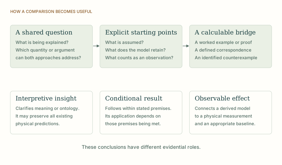
- Three different uses of temporal direction
- The useful synthesis


The forward and backward branches of a closed-time contour are a calculation of one physical quantum process. This article derives their origin from density-matrix evolution, explains their usefulness for DTT source models, and distinguishes contour bookkeeping, thermodynamic arrows and genuinely different operational roles for generation and completion.
To calculate an expectation value out of equilibrium, quantum theory evolves a density operator with U on one side and U† on the other. A path integral represents those two factors with a forward and a backward contour branch. The doubled fields keep track of amplitudes and their conjugates; they do not assert that a laboratory evolves through two independent physical times.
This makes the Schwinger–Keldysh formalism useful for DTT but not automatic evidence for it. A source can have unobserved internal work and an accessible record, while the contour is a mathematical device for computing correlations of that process. Their roles must be connected by an explicit model rather than equated because both descriptions contain a pair. [2]
The Single Monad Model begins with one nonspatial generative source. The Duality of Time Theory distinguishes the source’s inner production from the outer order in which completed records become accessible. Its six inner levels are nested functional roles of one process: a higher role organizes lower-level work. The seventh is the completion or observation interface. They are neither six independent clocks nor six additional time coordinates.
This distinction supplies a useful research question: which features of an observed world can follow from the way a source produces, retains and releases information? A concrete answer needs a state space, an autonomous update, retained memory and a rule connecting completion to an accessible measurement. In the constructions discussed here, those mathematical ingredients are stated explicitly. A successful finite example establishes what its specified mechanism can do; further arguments connect it to physical particles, spacetime or universal laws. [1]
Let H=ℏωZ/2 and prepare |+x⟩. The evolved density matrix is ρ(t)=U(t)ρ(0)U†(t), where U=exp(−iωtZ/2). Its upper off-diagonal entry becomes e^{−iωt}/2. Taking the trace with X gives ⟨X⟩=cosωt, and with Y gives sinωt in the corresponding convention.
The factors U and U† are both needed to obtain a real normalized expectation from amplitudes. Their occurrence does not mean that the qubit first travels forward in physical time and then comes back. Indeed Tr[UρU†]=Trρ=1 expresses probability conservation. In a generating-functional formulation with identical sources on the two contour branches, the analogous normalization is Z[J,J]=1. A valid DTT effective action written on this contour should preserve that identity when no outcome is postselected. [2]
ω is an angular frequency and t a single physical time. Contour sources J label external couplings, not additional clocks.
The formalism separates response from fluctuations. A retarded correlator vanishes before the perturbing operation in its specified causal ordering, while a fluctuation correlator describes statistical variation of observables. Integrating out an environment can produce dissipation and noise terms in an effective action. These terms have consistency conditions inherited from the full normalized dynamics.
DTT can use this machinery to calculate how hidden source variables affect completed records. It could derive a memory kernel or a phase lag and then compare it with a physically measured response. That is more specific than assigning one contour branch to inner time and the other to outer time. Such an assignment would need to explain why the conjugate branch, which is present in ordinary probability calculations, has acquired a new physical observable. [2] [3]
A contour orientation, a thermodynamic arrow and an ordering of released records are different structures. Reversing the contour is part of organizing an amplitude calculation. Reversing a thermodynamic process concerns a protocol and its probability distribution. Reversing the order of publicly available records concerns the physical dynamics of memory and observation.
The source programme can investigate whether one microscopic mechanism relates the last two, but the first does not establish that relation by itself. Similarly, a Wick rotation or an exchange of real and imaginary variables is an analytic operation unless an operational clock and evolution law give it physical meaning. The ordinary complex unit controlling quantum phase remains distinct from a split-complex unit used to represent hyperbolic temporal geometry. [2] [4]
The strongest connection is methodological: an explicit DTT source action can be placed on a closed-time contour, inaccessible registers can be integrated out and the resulting record response can be calculated. The formalism then tests whether the proposed effective dynamics preserves normalization, causal response and sensible noise correlations.
A new result would be a constrained kernel or fluctuation–response relation derived from the source’s nested organization and independent physical parameters. If the action is chosen freely to reproduce a desired curve, the contour calculation verifies that chosen model but does not explain its selection. This distinction lets DTT use a powerful established technique while keeping its proposed temporal ontology separate from the bookkeeping that the technique already requires. [2] [3]
THE SAME QUESTION, DIFFERENT STARTING POINTS
| Question | SMM/DTT | Schwinger–Keldysh contour |
|---|---|---|
| Meaning of the pair | Inner generation and outer completion are distinct physical roles only when their observables and access rules are specified. | Forward and backward contour branches encode U and U† for one physical process. |
| Observable target | A source model can predict a memory kernel, response or phase lag. | Closed-time methods calculate response and fluctuations from a stated action. |
| Normalization | Unconditioned completion dynamics must preserve normalized probabilities. | The contour satisfies Z[J,J]=1 under matching sources. |
KEEP THE CONNECTION
Connects this comparison with the author’s underlying construction.
Connects this comparison with the author’s underlying construction.
Connects this comparison with the author’s underlying construction.
Connects this comparison with the author’s underlying construction.
Connects the comparison to the programme’s current statement of results and assumptions.
References support the comparator and the specific mathematical or interpretive claims indicated. SMM/DTT connections are developed in the analysis above.
How these comparisons distinguish premises, results and physical claims
SMONAD
Share this page, or keep a clear reference to the work you are reading.
Use this reference for the explanation on this page. “n.d.” means its first publication date is not specified; the update date is recorded separately.