

A shared operator creates linked predictions
An atom provides several possible comparisons: its energy levels, spatial probability distribution, momentum variance, and response to perturbations. A common model is informative when one parameter set predicts these together. Fitting a separate scale to each observable can conceal a failure of that common description.
The laboratory supplies the relative-coordinate Hamiltonian H=p²/(2μ)−αℏc/r for two point particles with reduced mass μ. It assumes the nonrelativistic Coulomb regime and standard quantum state rules. Spin, radiative effects, nuclear size, and relativistic corrections are outside this baseline.
The existing SMONAD atomic guide derives the normalized ground-state profile and its linked scales. The illustrated experiment isolates one exact relation so its dependencies are visible. SMM/DTT would add a source derivation of the effective Hamiltonian and its independently normalized parameters; the baseline alone does not provide that derivation. [X10] [B16]
Change the coupling and preserve the kinetic dictionary
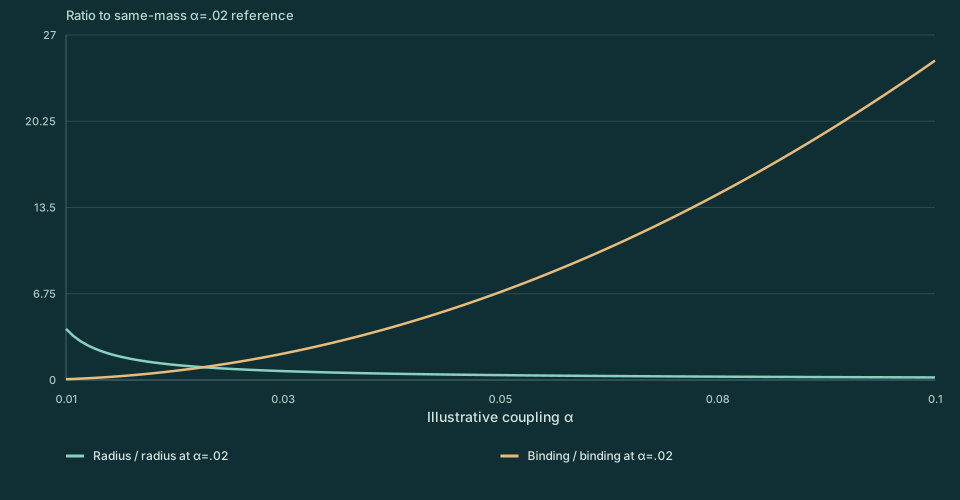
Vary the supplied positive coupling α and reduced mass μ/mₑ. The two curves show radius and binding as ratios to their values at α=0.02 for the same mass. The numerical readout separately gives radius in reduced electron-Compton lengths and binding in electron rest energies. At fixed μ, doubling α halves a and multiplies B by four.
Interactive calculation
Play scans Illustrative coupling α. Step advances it. No animation starts automatically.
Enable JavaScript for adjustable values. The static figure and worked calculation remain available.
In scaled units with ℏ=c=mₑ=1 and μ/mₑ=1, choosing α=0.02 gives a=50 and B=0.0002. Choosing α=0.04 gives a=25 and B=0.0008. Both have Ba²=0.5. These deliberately illustrative dimensionless parameters are not a precision model of measured hydrogen and are not independently derived constants.
Derive the radius–energy identity
The factors of α and c cancel in the product. Its dimensions are energy times length squared, matching ℏ²/μ. The identity therefore compares an interaction-sensitive radius and energy through an independently fixed kinetic coefficient.
The ground-state wavefunction is ψ(r)=exp(−r/a)/√(πa³). It is normalizable because its radial shell probability integrates to one: P(r)=4r²exp(−2r/a)/a³. The parameter a is the most probable radial separation, while the mean separation is 3a/2. It is not a sharply defined orbit radius or the nuclear charge radius measured in a different experiment.
The ratio ΔE₂₃/ΔE₁₂=5/27 cancels B. A level table also enforces ΔE₁₃=ΔE₁₂+ΔE₂₃. These checks require a consistent transition convention. Converting energy to ordinary frequency uses ΔE/h, whereas angular frequency uses ΔE/ℏ.
If only μ changes at fixed α, then a scales as μ⁻¹ and B as μ. The product Ba² therefore scales as μ⁻¹ rather than remaining a universal numerical constant. That distinction prevents a change of isotope or effective kinetic mass from being mistaken for a failure of the fixed-mass identity.
Use the identity as a check with independent inputs
First define which spatial observable estimates a, which spectral interval estimates B, and how the kinetic coefficient is independently determined. If a is calculated from the same fitted B using the identity, their agreement is algebraic rather than an independent observation. If both are obtained through one analysis, their covariance must be included.
A finite source calculation can be tested against the normalized profile and multiple moments as well as the energy. Its grid, finite volume, and state preparation contribute errors that should decrease under a specified refinement. Good agreement at one radius does not establish convergence of an entire bound state.
The book's common-dictionary requirement is especially useful here: the action scale, clock, mass assignment, and spatial calibration must be held consistent across the calculations. The same input cannot be silently refitted when a second observable is examined. [X02] [X03] [X05]
Every positive Coulomb coupling in this ideal family binds. Binding and the radius–energy identity therefore do not single out 1/137 or any other value. A source-selected coupling would make the atomic relations additional predictions only after the upstream selection and physical matching are independent.
Continue to isotope comparison to vary the nuclear mass while keeping the same electronic interaction law. For the spatial interpretation, see the Matter hydrogen laboratory.