


A useful test begins before the reserved data are examined
A model adjusted after every comparison can describe a dataset without predicting the next observation. A stronger protocol fixes the preparation, mathematical form, fitting rule, and calibration data before evaluating a reserved comparison. The SMM/DTT book illustrates this with dispersion and memory models whose same parameters must work across different settings. [X04] [X05]
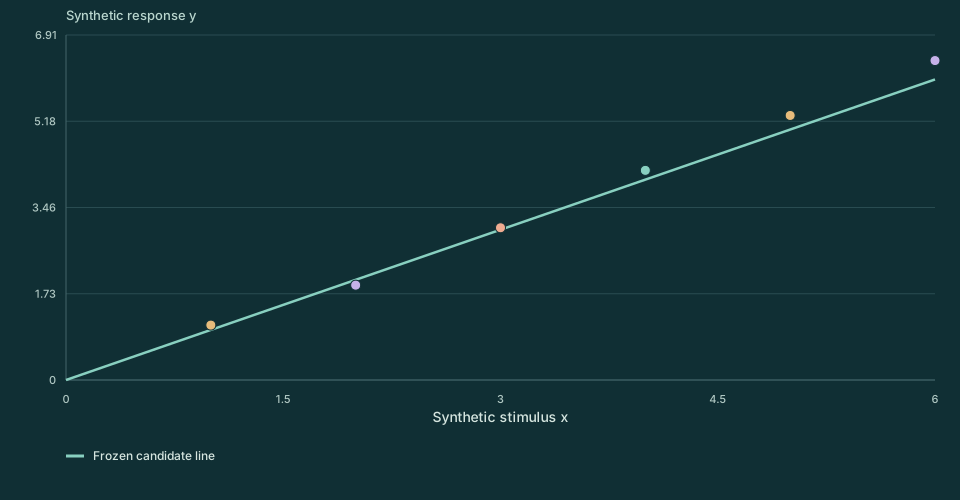
This laboratory uses a deliberately synthetic six-point dataset. The inputs are x=1,2,3,4,5,6 and the outputs are y=1.1,1.9,3.05,4.2,5.3,6.4. No physical measurement produced these values. The first three points form the calibration set; the final three form the reserved set.
The candidate model is y=βx with zero intercept fixed in advance. Its calibration slope is determined by least squares on the first three points only. The later points test that particular restriction. Choosing a zero intercept is itself an assumption about the origin and offset; it is not a harmless plotting convention.
Compare calibration error with reserved error
With slope correction Δa=0, inspect the frozen line and the two groups of points. The fitted slope is approximately 1.00357143. Its first three residuals have mixed signs, while all three reserved residuals are positive and grow with x. The root-mean-square calibration residual is about 0.08626; the reserved value is about 0.29292.
Interactive calculation
Play scans Candidate slope correction Δa. Step advances it. No animation starts automatically.
Enable JavaScript for adjustable values. The static figure and worked calculation remain available.
Change Δa to explore a candidate slope β̂+Δa, or change the assumed common uncertainty σ. The displayed χ² summaries sum squared residuals divided by σ² in each group. A slope chosen after looking at the reserved points has used those points for fitting. It is no longer the original reserved prediction and needs a new untouched comparison to test it.
Calculate the frozen prediction once
Differentiating the calibration sum of squares Σ(yᵢ−βxᵢ)² gives the normal equation βΣxᵢ²=Σxᵢyᵢ. The fitted slope is therefore fixed by the declared three observations and model form. It is not recalculated when the reserved points are displayed.
Residuals are observed or supplied outputs minus model predictions. Their sign and dependence on x contain information that one overall fit score can hide. The NIST model-validation guidance emphasizes checking residual structure rather than relying on a large coefficient of determination alone. [X08]
If each response had independently known Gaussian variance σ² and the x values were exact, the calibration slope variance would be σ²/14. Prediction errors at reserved points would share the covariance xⱼxₖσ²/14 from that same estimated slope. Each individual error would also include its own response variance.
Consequently, dividing each residual by a chosen σ is an illustrative scale comparison, not automatically a complete joint significance test. Uncertain x values, an uncertain offset, heterogeneous noise, or temporal correlation change the model. The synthetic dataset does not independently establish any of those noise properties.
What a failed prediction should change
The growing reserved residual suggests that the through-origin linear rule is inadequate for this constructed example over the full range. Several explanations could fit the pattern: curvature, a gain drift, an offset, or a different dependence. Six synthetic points cannot identify a unique physical mechanism.
A revision should state which assumption changed and why, then define a new calibration and reserved comparison. Adding parameters until the displayed points are reproduced measures descriptive flexibility. It does not create independent evidence for the revised mechanism.
A source theory becomes stronger when it fixes relations among parameters before the test, thereby reducing the allowed patterns. The experimental programme asks for precisely this transition from an interpretable construction to predictions that can disagree with alternatives. [X07] [P01]
Keep calibration uncertainty, selection rules, and all inspected comparisons in the record. For empirical data, the choice of what to reserve should precede inspection, and testing many alternatives requires an appropriate statistical treatment. Continue to nuisance directions to determine whether the proposed pattern is distinguishable even with perfect agreement or much greater precision.