

More observables help only when they add new dependence
A small unexplained residual is not automatically a new physical effect. It may be reproduced by a calibration shift, an uncertain conventional coefficient, or another permitted model parameter. To design a discriminating experiment, compare the proposed signal pattern with the patterns generated by these nuisance parameters.
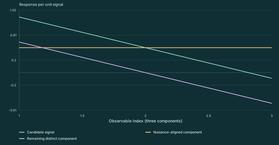
The laboratory has three observables. A common additive nuisance changes them along n=(1,1,1). The distinctive reference contrast is s=(1,0,−1). These vectors are perpendicular. The candidate unit signal sθ rotates continuously from the normalized common direction toward the normalized contrast.
The mean response is y=A sθ+B n, where A is the amplitude of interest and B is an unrestricted nuisance offset. The angle θ is a supplied design parameter. This finite example illustrates identifiability; it is not a computed SMM/DTT spectral pattern or evidence from three actual transitions.
Keep the signal size fixed and vary its distinctness
Change θ. At θ=0°, the candidate signal is proportional to the nuisance direction. Any change in A can be absorbed into B, so the two amplitudes cannot be separated from these observations alone. At θ=90°, the signal is fully orthogonal to the nuisance and remains after subtracting a common offset.
Interactive calculation
Play scans Signal angle θ (degrees). Step advances it. No animation starts automatically.
Enable JavaScript for adjustable values. The static figure and worked calculation remain available.
At θ=30°, only half of the unit signal length survives nuisance removal. With independent equal output uncertainty σ=0.1, the corresponding local information for A is 25, compared with 100 at θ=90°. Halving the distinct signal component reduces the information by a factor of four.
Project out the nuisance direction
The candidate vector has norm one at every angle because n̄ and s̄ are orthonormal. The component distinguishable from an arbitrary common offset has norm |sinθ|. A large total response is therefore compatible with almost no information about its separate source amplitude.
This is the profiled Fisher information for a linear Gaussian model with known covariance σ²I and a free nuisance amplitude. It can also be obtained as the Schur complement of the two-parameter information matrix. At θ=0, it vanishes exactly; reducing σ cannot remove the exact degeneracy.
For θ≠0, the best linear unbiased amplitude estimate in this model has variance σ²/sin²θ. Near zero, the variance becomes large even though the parameters are formally identifiable. This is the quantitative difference between a nonzero determinant and a useful experimental design.
The contrast d cancels B directly. Its noise variance is σ² when the two corresponding errors are independent and each has variance σ². Correlated or unequal errors require their covariance; the optimal projection is then performed in the inverse-covariance metric rather than the ordinary Euclidean one.
A fourth measurement that repeats the same proportional pattern can improve precision, but it does not break an exact signal–nuisance degeneracy. A measurement with different physical dependence, or an independent restriction on B, can. The source of the extra information must be identified rather than counted twice.
Choose a comparison that can identify a mechanism
For a real protocol, calculate the sensitivity of every selected observable to the proposed source parameter and to each relevant conventional input. Include shared calibration, mass, nuclear, environmental, and apparatus uncertainties as appropriate. A full-rank response matrix can still be poorly conditioned, so inspect its small singular values and expected uncertainties.
If a source proposal predicts a relation among several effects, use that relation to define a restricted signal pattern before examining the data. An independently fixed relation can reduce the number of adjustable directions. Allowing separate coefficients for every residual can make almost any pattern fit, removing the intended test.
The common-dictionary and explicit-alternative requirements in the books lead naturally to this design question. A shared source should constrain several outputs with fewer independently chosen inputs, while the measurement model carries its uncertainties honestly. [X02] [X03] [X05] [X09]
Return to the experimental guides for connected protocols, or use the research dependency map to follow which theoretical inputs each comparison requires. These laboratories identify mathematical opportunities and obstructions; they do not claim that a new physical residual has been detected.