

An accurate fit can still leave the parameter unknown
Suppose an experiment produces a response proportional to a controlled input x. A proposed coupling α affects the response, but so does an instrument gain g. In the laboratory model y=gαx, the full noiseless curve determines A=gα. It does not separately determine α and g.
This is a minimal example of a normalization problem. The book emphasizes that a carrier dimension or an integer count does not by itself fix a physical response: source strength and operator normalization also enter. The published OMS reconstruction discusses this transition from finite structure to normalized response. [X06] [P01] [A02]
The symbol α here denotes a positive model coupling. The simple linear response is an illustrative identification problem, not a complete electromagnetic experiment or a claim that every physical measurement of the fine-structure constant contains an unconstrained gain. Real determinations specify and independently constrain their measurement model.
Change the parameters while keeping the observable fixed
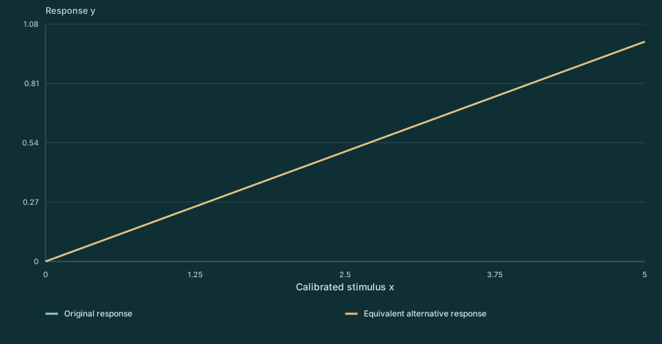
Vary the gain and coupling and inspect the response slope. A gain twice as large together with a coupling half as large produces exactly the same y at every x. The alternative-gain control automatically calculates the corresponding alternative coupling, displaying two coincident curves. No additional x points can distinguish those pairs within this model.
Interactive calculation
Change the inputs to compare the model outputs.
Enable JavaScript for adjustable values. The static figure and worked calculation remain available.
For example, (g,α)=(2,0.25), (1,0.5), and (0.5,1) all give y=0.5x. If an independent reference establishes g=2, that observed slope A=0.5 implies α=0.25. Calling the same response curve a gain calibration and then using it again to claim an independent coupling prediction would count the information twice.
Write the ambiguity as an exact symmetry
The set of indistinguishable parameter pairs is a hyperbola in the positive gain–coupling plane. The parameterization has two coordinates, but the data depend on only one combination. This remains true with infinitely many exact observations of x and y.
The sensitivity columns are proportional. Consequently, the two-parameter information matrix has rank one for this response alone. Increasing precision sharpens the estimate of the product A, while the ambiguity along constant-product pairs remains.
Once g is independently calibrated, ordinary uncertainty propagation gives an approximate relative variance for α. To first order, Var(α)/α²≈Var(A)/A²+Var(g)/g²−2Cov(A,g)/(Ag). The covariance term disappears only when the corresponding estimates are independent. Shared reference standards or shared data can correlate them.
The first-order expression assumes uncertainty small enough for linearization around nonzero g and A. Wider or asymmetric uncertainty may require propagating the full measurement model. Reporting only the formal fit error in A would omit the calibration contribution.
A second observable can also break the degeneracy if its dependence is independent. For example, a separately established response z=gx determines g from its slope. Another curve proportional to gα with a known prefactor supplies precision but no new parameter direction. The functional dependence, not merely the number of graphs, determines identifiability.
The alternative gain is a mathematical comparison parameter. Its automatically calculated α′ may differ from the original coupling while leaving every curve point unchanged; that coincidence is the result being tested, not a display error.
Connect a structural proposal to an independent test
A source-derived α would have to be fixed upstream of the reserved response measurement, with the physical source, normalization, and energy regime specified. The same parameter should predict more than one observable through a shared dictionary. Changing the gain or coupling independently for every channel would remove that cross-check. [X02] [X03]
Calibration is useful physical work. The crucial distinction is which information determines the inputs and which observations remain predictions afterward. A clear dependency record states the calibration dataset, uncertainty, nuisance parameters, and all later uses of the result. Metrology guidance provides the language for these measurement models and correlated inputs. [X09]
Continue to atomic consistency, where one supplied Coulomb coupling predicts several linked scales. Their relationship is a stronger check than a single fitted number, while still leaving the independent origin of the coupling to be established.