
A static response remains unchanged when its source and stiffness are transformed together. The same symmetry still permits different response strengths, showing why covariance alone cannot select a physical coupling or constant.
Transform the complete description
Represent a real finite state by a vector x. Under an orthogonal change of components x′=Rx, a quadratic energy xᵀKx/2 has the same meaning if K′=RKRᵀ. A source term fᵀx must similarly use f′=Rf. Transforming one symbol while keeping the others fixed usually changes the model rather than merely changing its description.
This principle is especially useful for SMM/DTT. A source carrier, its completion tests and its physical readouts must transform together. Agreement of two formulas written in different frames is meaningful only after their states, parameters and measurements have been translated consistently.
Derive an invariant capacity
Assume K is positive definite and minimize E(x)=xᵀKx/2−fᵀx. Differentiation gives Kx=f, so the equilibrium response is x*=K⁻¹f. The scalar C=fᵀK⁻¹f measures the response in the applied-source direction.
C′=f′ᵀK′−1f′=fᵀK⁻¹f=C.
The equality follows from RᵀR=I. It is exact and does not depend on K being isotropic. An anisotropic system can have a coordinate-independent description because the apparatus orientation and its response matrix are transformed together.
Worked example: a quarter-turn changes components
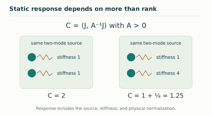
Take K=diag(1,4) and f=(1,1). The capacity is 1+1/4=5/4. A quarter-turn R maps f to (−1,1) and K to diag(4,1). Repeating the calculation gives 1/4+1=5/4.
Now replace K by the identity while keeping the physical source fixed. The capacity becomes two. This second operation changes the stiffness, not the coordinate basis. Equal carrier dimensions therefore do not imply equal response. A physical constant cannot be inferred from a mode count without selecting the source, the stiffness and their normalization.
One invariant need not determine the whole object
The matrices diag(1,3) and diag(2,2) both have trace four, yet their determinants are three and four and their spectra differ. Trace is invariant under similarity, but it is not a complete description of a matrix. Choosing a limited family of invariant tests can merge physically distinct possibilities.
The same issue occurs for completed records. A loop trace, a determinant degree or a total mode count retains particular information. The source programme must establish which invariant its apparatus measures and whether that invariant suffices for later predictions. More invariants may be required without changing the proposed unity of the source.
Transport between receivers differs from one fixed representation
A receiver may depend on an auxiliary flag: a line inside a plane inside a three-dimensional readout. Rotations can transport the entire receiver and its response data between flags. This can define a covariant family even when no single fixed receiver carries the stronger rotation action one might have expected.
The linked rank-137 construction gives a precise example. Under its unoriented-flag convention, three conjugate half-turns would need equal characters in any fixed SO(3) representation, but their natural stabilizer traces are 1,−7,−7. That obstructs the fixed representation. A transported scalar capacity can nevertheless remain flag independent when the base response data satisfy the required stabilizer conditions.
What the surviving symmetry leaves unfixed
Even full rotational isotropy allows a positive stiffness K=κI with any κ>0. It removes directional preference without fixing the magnitude of the response. In a d-dimensional model with a source of squared norm d, the capacity is d/κ.
For SMM/DTT constants work, this distinction preserves the meaning of structural integers. A receiver rank such as 137 can be exact within its selected construction while its physical response depends on an independently supplied κ. Symmetry can constrain the form of the law before it constrains, or fails to constrain, the remaining scale.
A stronger invariant prediction
The next useful result would derive a relation among independently measured responses from one source update. For example, the same microscopic parameter might control stiffness, clock rate and a transport coefficient, leaving a dimensionless ratio fixed as the parameter varies.
The six nested inner roles could contribute by enforcing a shared resource or composition identity, while outer completion defines the readable quantities. The calculation should transform all apparatus data consistently, then change a physical parameter and show which prediction remains. This separates a universal relation from an invariant rewriting of a model whose coefficients were freely chosen.
Continue with the articles
- Trace-sector response and the Schur complement
Introduce the reduction that gives capacity N/s under ordinary trace coupling. Show how hidden response sectors can affect an apparently simple scalar observable.
- The conditional ideal value one over 137
Summarize the extra normalization and electromagnetic matching needed for the ideal model coupling. Explain why the draft’s alpha-zero notation does not denote the measured low-energy constant.
- A flag-independent response without one fixed rotation action
Explain the draft’s distinction between covariantly transported response and a single fixed rotation representation. A useful invariant can survive even when a stronger representation requirement fails.
- Two phase actions and determinant closure
Compare the inherited polynomial phase with the selected coherent-output phase. Explain why determinant closure can produce a 137-fold condition only after the stated phase identifications.
- A dependency map for physical constants
Introduce the constants program as a chain from completion dynamics to response and then physical matching. Identify which quantities are structural, calibrated, or still free.
- What the holonomy Hessian does and does not contain
Explore the exact trace structure of the response near identity holonomy. Explain why the absence of an independent squared-trace term matters for the model’s coefficient relations.