


Visual tour · Research and comparison
From structural counts to physical tests
Follow receiver modes, the conditional count 137, response normalization and hydrogen benchmarks toward a reproducible comparison with observations.
A structural calculation becomes physically informative when its quantities are connected to a declared preparation, an observable and a common set of units. This route follows those connections from finite receiver modes to atomic benchmarks.
The diagrams contain exact results within specified constructions and proposed ways to test a broader source model. Keep the physical matching assumptions visible as you move between them; the same parameters must support all linked comparisons.
Stop 1 of 6
Identify what the receiver is counting
Four diagonal and six symmetric off-diagonal basis elements give a ten-dimensional symmetric receiver space. Mirrored off-diagonal entries belong to one mode. The count is exact once that space has been chosen; the physical argument must explain which histories this receiver distinguishes and why those are the admitted tests.
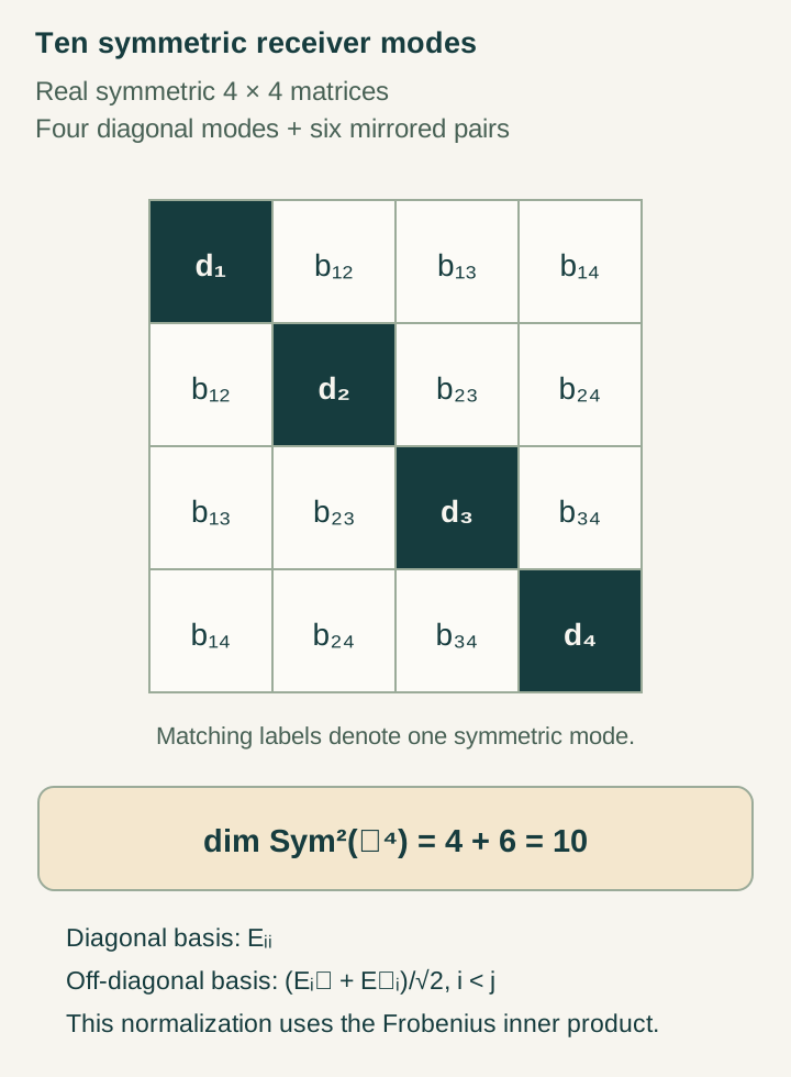
Four diagonal and six normalized off-diagonal basis matrices span the ten-dimensional space Sym²(ℝ⁴). Matching mirrored entries describe one symmetric mode, while choosing this space as a physical receiver is a modeling step.
Find this figure in the galleryStop 2 of 6
Follow the disjoint sectors to 137 records
The three terminal sectors contain 100, 30 and 7 distinguishable records. Their disjointness makes the total 137 in the specified grammar. Read the proportional bar as a count of retained alternatives; sampling probabilities and interaction strengths still require their own definitions.
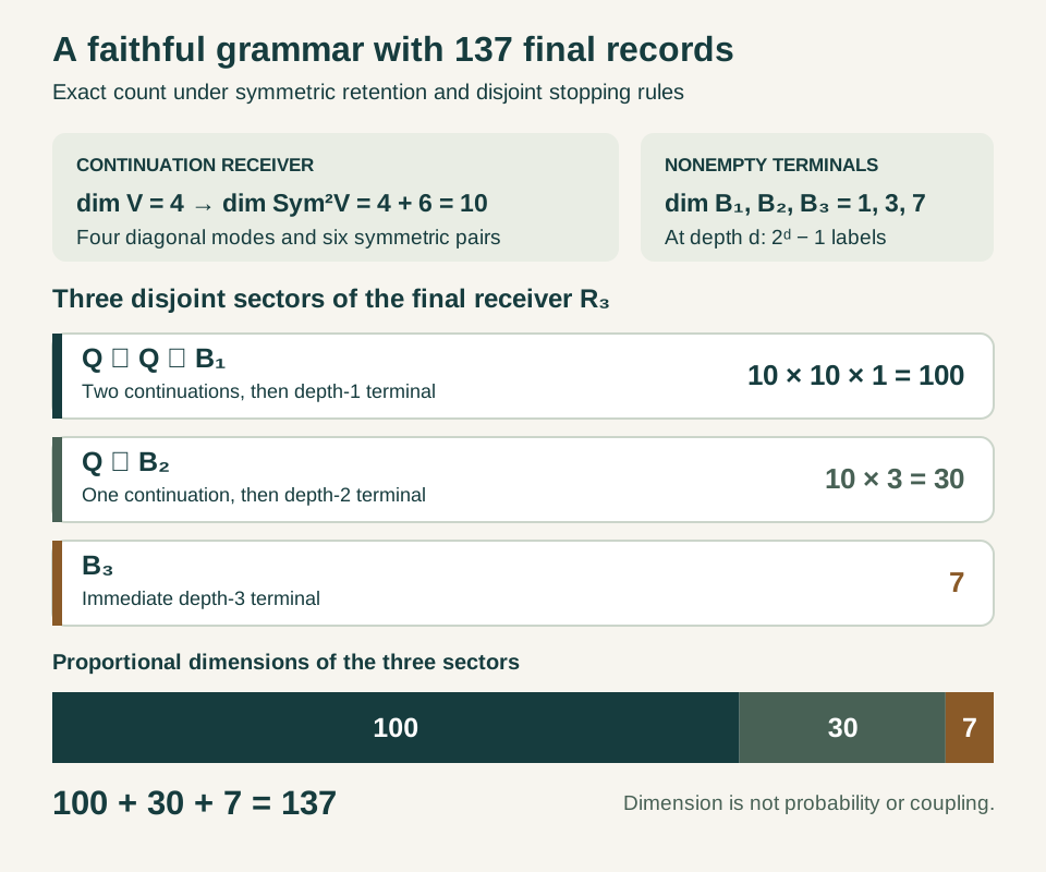
The ten-mode continuation receiver and disjoint terminal sectors produce 100, 30 and 7 records, with a proportional bar showing their exact sum.
Find this figure in the galleryStop 3 of 6
Allow hidden modes to change the response
For the stated quadratic example, E(z) = 1 + z + z², allowing the hidden coordinate to relax moves the minimum from the frozen value 1 to 3/4 at z = −1/2. The calculation shows why a physical response depends on stiffness, probe normalization and accessible relaxation as well as record count.
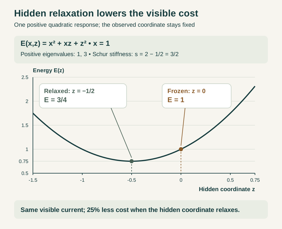
An exact positive quadratic energy at fixed visible coordinate shows how hidden relaxation changes the minimum from one to three quarters.
Find this figure in the galleryStop 4 of 6
Require one coupling to organize several atomic scales
In the supplied Coulomb model, multiplying the positive coupling by t changes the radius by 1/t, the relative RMS speed by t and the binding-energy magnitude by t². These linked consequences are exact within that Hamiltonian and convention. A source-derived coupling would have to reproduce them together with the required masses, action and propagation scale.
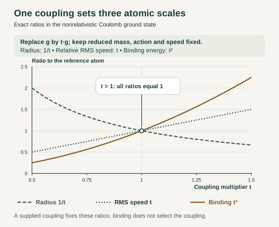
Exact Coulomb-model curves show how the radius, relative RMS speed and binding change together when the supplied coupling is multiplied by t.
Find this figure in the galleryStop 5 of 6
Freeze the baseline before reading residuals
The proposed comparison connects several atomic probes to one fixed baseline. Residuals become informative through their shared pattern, independent sensitivities and uncertainty covariance. Multiple lines that repeat the same constraint do not supply independent tests, and a fit made after seeing the target data must be distinguished from a prediction.
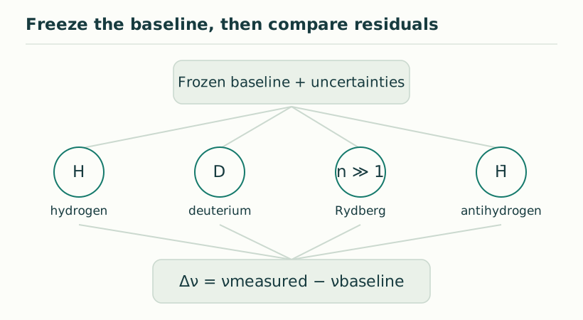
A fixed baseline links hydrogen, isotope, Rydberg, and antihydrogen comparisons before residuals are assessed. The schematic describes a test design; nuisance cancellation depends on a specified covariance model.
Find this figure in the galleryStop 6 of 6
Choose the next bridge to establish
Trace a path from the common source to locality, clocks, propagation, composition and observable predictions. Each arrow names work needed to join the constructions into one physical account. The claim map records the role and assumptions of the statements; the open problems identify concrete mathematical and operational targets for collaboration.
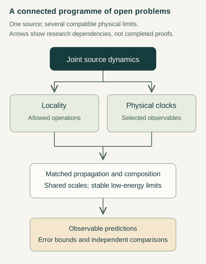
Joint source dynamics connects research on locality and clocks to propagation, composition, and observable predictions. Each arrow names an obligation requiring a mathematical or operational construction, with error bounds at the comparison stage.
Find this figure in the gallery