


Visual tour · Geometry and clocks
From relations to geometry and physical clocks
Read six diagrams connecting local moves, causal cones, calibration, proper time and retained memory, with links to the underlying calculations.
A drawing can arrange records on a page without yet assigning them a physical distance or duration. This tour follows the additional rules that make geometric comparisons and clock readings meaningful.
The sequence moves between exact mathematical examples and the source-model requirements they illuminate. At each stop, ask what is supplied, what is calculated and how a physical instrument could realize the comparison.
Stop 1 of 6
Let permitted moves define distance
Count the allowed steps along the upper chain, then include the extra edge in the lower graph. The endpoint distance changes from four to one even though the page layout remains similar. This example makes adjacency operational: a distance law depends on allowed comparisons and their calibrated costs.
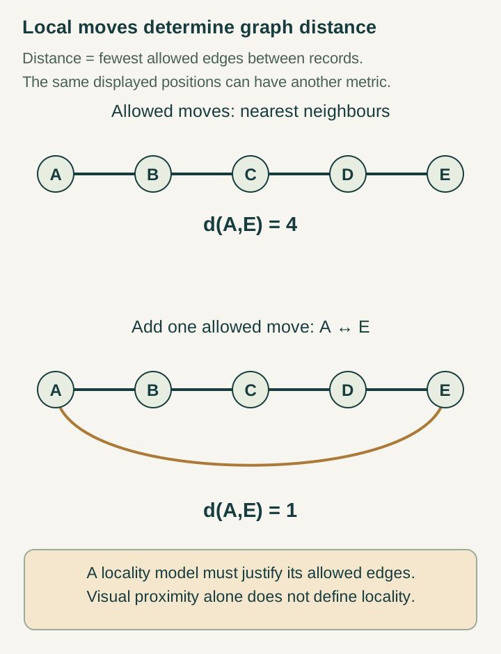
A five-node chain has endpoint distance four; adding an allowed direct move reduces that distance to one. Graph distance is fixed by the permitted elementary operations, independently of the drawing's Euclidean layout.
Find this figure in the galleryStop 2 of 6
Recognize the cone inside the algebra
For a two-by-two Hermitian record X = tI + x·σ, the determinant is t² − ‖x‖² and positivity requires t ≥ ‖x‖. The shaded section therefore has Lorentz-cone shape. The identity is exact for the stated representation; a physical reconstruction must also identify its records, allowed transformations and clock interpretation.
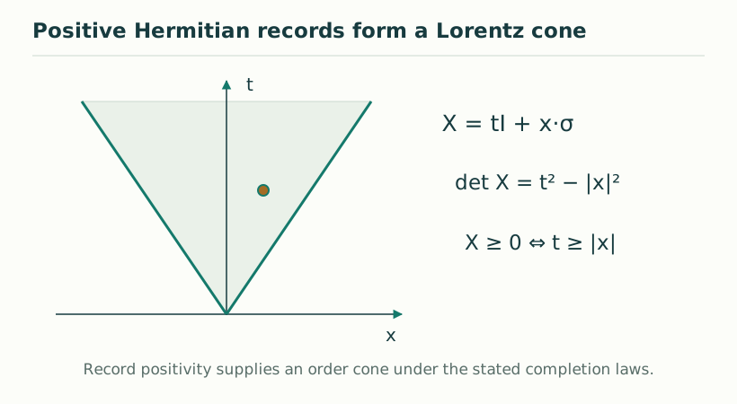
For X = tI + x·σ, det X = t² − ∥x∥² and positivity is equivalent to t ≥ ∥x∥. The drawing is a two-dimensional section of this four-dimensional positive Hermitian cone.
Find this figure in the galleryStop 3 of 6
Add the scale that causal shape leaves open
The two cones preserve the same causal shape while their length standards differ. A positive rescaling preserves which directions are null, but changes volumes and elapsed proper times. Read the ruler and volume cell as additional calibration data whose agreement across measurement protocols needs to be established.
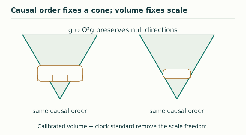
A causal cone fixes conformal relations, while an independent volume or ruler calibration fixes scale. Realizing those relations as physical boosts additionally requires compatible clocks and detectors.
Find this figure in the galleryStop 4 of 6
Specify what a protected clock responds to
The commuting square compares branch activity before and after an admitted clock test. Under the stated coupling and observation assumptions, branching leaves the clock statistic unchanged while resolution evolution can change it. Delayed tests matter because a distinction invisible in the immediate display can become observable later.
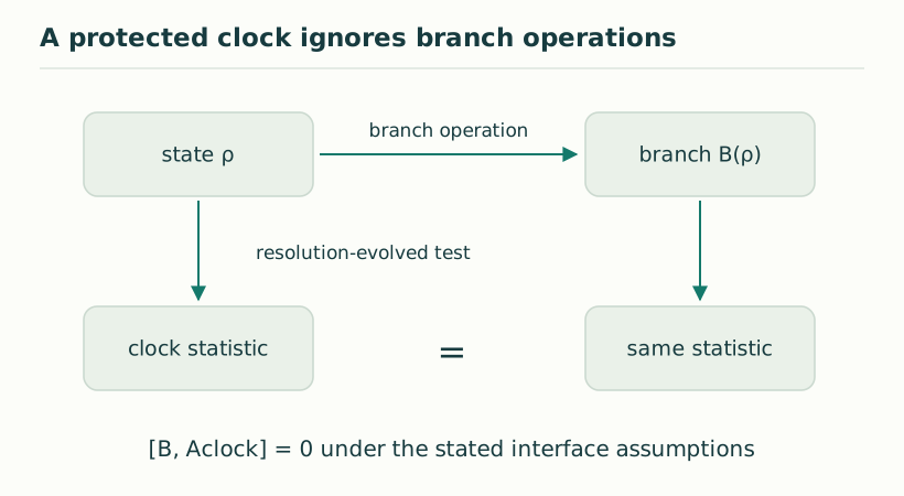
A commuting interface makes an admitted clock statistic insensitive to specified branch operations. Resolution evolution can still change the reading, so the result identifies a protected clock under stated coupling assumptions.
Find this figure in the galleryStop 5 of 6
Compare the duration along each worldline
In the displayed flat-spacetime example, the straight history accumulates five proper-time units and the two-leg history accumulates four, with c = 1 and an idealized turnaround. These are standard interval calculations for the supplied paths. A DTT realization must show how its material clock reproduces the same path-dependent reading.
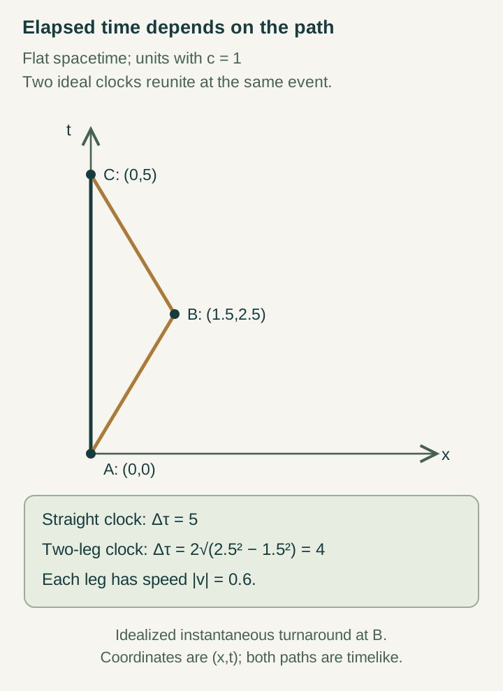
A straight worldline records five proper-time units while the displayed two-leg path records four in units c = 1. The exact piecewise-inertial comparison idealizes the turnaround and follows from integrating each path's interval.
Find this figure in the galleryStop 6 of 6
Track the memory left by an eliminated variable
Start with the coupled variables, then follow the elimination of the relaxing hidden variable. Its past influence survives as an exponential memory kernel in the reduced equation. The example shows how a local evolution of the full state can yield a history-dependent description of the observed part.
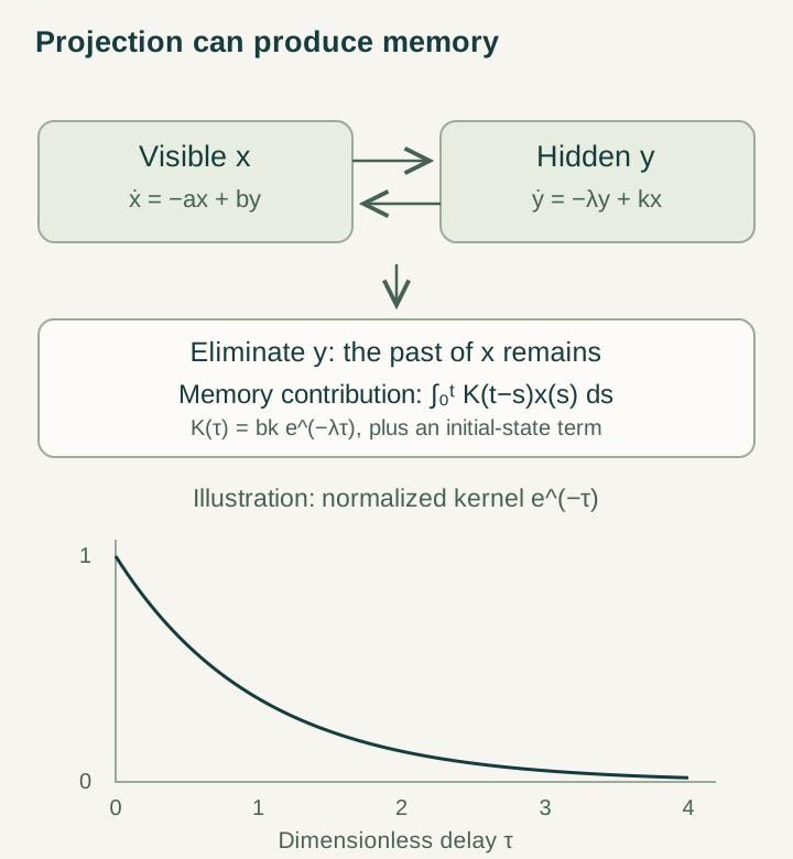
A two-variable local system becomes history-dependent after its relaxing hidden variable is eliminated. The exponential kernel records the exact delayed contribution under the specified linear dynamics.
Find this figure in the gallery