
A locally calibrated frame supplies a metric, while transport around loops and relative free fall reveal curvature. Obtaining that geometry is distinct from deriving Einstein's field equation, its matter coupling and its physical constants.
Build geometry from local comparisons
At each completed event, suppose physical instruments identify one duration direction and three independent displacement directions. A calibrated local frame translates coordinate increments into those readings. With Lorentzian calibration, the metric is assembled as gμν=ηabeaμebν, where η has signature (−,+,+,+).
The frame fields e carry the connection between coordinates and apparatus. In SMM/DTT, a source model would generate these local comparison rules from retained records and their transport. A rank-three readout plus one clock direction is the starting structure; compatible smooth attachment and calibration are additional requirements before a spacetime metric is defined.
A varying completion rate as a metric candidate
A simple static candidate has line element ds²=−N(x)²c²dt²+hij(x)dxidxj. The positive lapse N gives stationary clock readings dτ=Ndt, while h determines spatial comparisons on the selected static slices.
DTT may interpret variation in N as variation in how a completed material clock accumulates duration relative to the chosen coordinate label. That interpretation becomes geometric only if matter propagation and signal comparisons use the same structure. An arbitrary position-dependent oscillator frequency does not automatically define gravity; it may instead be an ordinary external perturbation of one apparatus.
Worked example: two stationary clocks
Let a static region have N(A)=1 and N(B)=1.000002. Over the same coordinate interval, clock B accumulates 1.000002 times the proper duration of A. Its local rate is higher by two parts per million in this illustrative geometry.
For a stationary transmitted signal: νB/νA=N(A)/N(B).
The second relation follows because successive wave crests preserve their coordinate-time spacing in a static background, while local proper intervals differ. A signal emitted at A is therefore received at B with a slightly lower frequency relative to B's local clock. The lapse predicts both effects together.
Changing coordinates is not producing curvature
A metric can vary with position even in flat space. The ordinary Euclidean plane in polar coordinates has ds²=dr²+r²dφ². Its position-dependent coefficient r² records the coordinate choice, while its intrinsic curvature remains zero.
For a genuine curvature example, a sphere of radius R has geodesic circles of circumference C(r)=2πR sin(r/R). At small radius, C/(2πr)=1−r²/(6R²)+higher terms. A circle of geodesic radius R/10 has a ratio approximately 0.998334. This is an intrinsic comparison between radius and circumference. The sphere illustrates curvature mathematically; it is not being proposed as the physical spacetime metric.
Transport and tides reveal the invariant content
Comparing a vector transported along two different nearby routes can expose a mismatch governed by curvature. Similarly, neighbouring freely falling bodies can change their separation even when each has zero proper acceleration. These are operational ways to distinguish intrinsic geometry from coordinate artifacts.
In a record-based model, transport rules must specify how local frames and material orientations are compared across completed sites. The comparison around a small loop should converge consistently as the archive is refined. Arbitrary relabeling of sites must not change the result. This provides a direct SMM/DTT target: derive stable loop comparisons from the same source operations that generated local distances.
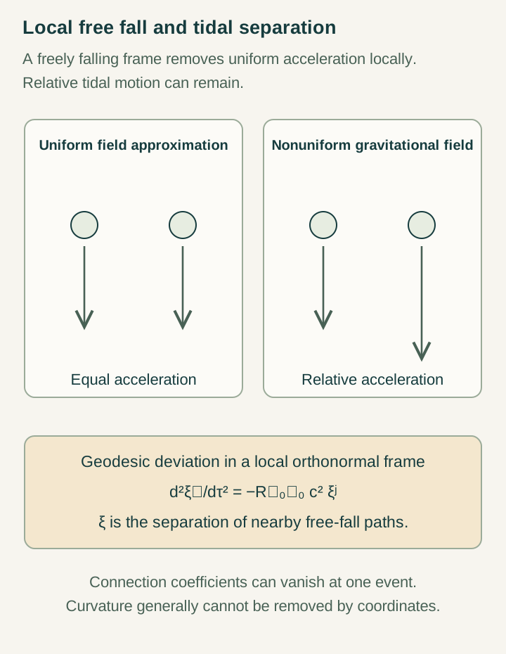
Open the full-size diagram →
Curvature still needs an evolution law
A Lorentzian metric determines curvature through differential geometry. Einstein's equation is the additional dynamical relation between that curvature and stress–energy:
It follows from the Einstein–Hilbert gravitational action with a specified matter action and coupling, under the appropriate variational treatment. Other covariant actions can produce different equations on the same kind of geometry. Thus deriving a cone, a density or a curved comparison metric does not alone derive Einstein dynamics, the value of G or the cosmological term Λ.
What temporal generation would have to supply
A source-level account should explain how the energy and correlations of persistent matter change the completed comparison structure. It needs a conservation law, a controlled large-scale limit and a common coupling between matter and geometry. The gravitational response must be calculated from the microscopic update rather than imposed after the metric has been reconstructed.
The six nested inner roles can organize local generation and the seventh can certify the resulting record. Their physical contribution would become sharper if the work needed to maintain a matter pattern altered nearby completion or comparison rules in a uniquely constrained way. That response could then be tested against the required weak-field and curvature laws.
A manageable next derivation
Begin with a weak, slowly varying background and two distinct matter carriers. Derive their clock redshift, free-fall acceleration and local propagation from the same update. Reconstruct a candidate metric from independent measurements and check whether it predicts all three responses without separate fitting.
Only then ask which effective action governs that metric and how stress–energy enters it. This order keeps the programme concrete: first operational geometry, then universal matter response, then gravitational dynamics. Agreement at the weak-field level would be a substantive step toward SMM/DTT gravity while leaving strong-field behavior and the full continuum field equation as explicit later targets.
Continue with the articles
- Relative and Curved Time
An introductory discussion of relative time and the geometric language of curvature. Prepare a careful comparison between historical temporal imagery and modern spacetime descriptions.
- From a cone inequality to a Lorentzian metric
Explain the construction of a Lorentzian metric from a positive spatial metric and a temporal one-form. Identify the signature and nondegeneracy conditions required by the model.
- A spectral triple as a reconstruction interface
Introduce the algebra, Hilbert space, and Dirac-type operator used by the temporal spectral model. Explain the different jobs of observables, states, and spectral data.
- Graph distance from a normalized spectral block
Introduce the graph-block construction whose Connes distance equals weighted shortest-path distance. Explain the normalization assumptions behind that equality.
- One clock direction plus three readout directions
Explain the rank-one clock and rank-three readout used in the conditional four-dimensional construction. Clarify why a soldering map is needed to identify them with tangent directions.
- Calibrating a conformal geometry
Explain why a causal cone fixes less than a fully scaled metric. Introduce the record-density and clock standards used to supply the remaining scale in the draft.
- What Lorentzian reconstruction leaves open
Summarize the boundary of the constraint-relative theorem. Recovering a causal geometry does not itself determine matter dynamics, the numerical limiting speed, or Einstein’s field equations.
- Four principles of quantum relativity: assumptions and consequences
Follow the four proposed principles through their mathematical dependencies. The guide connects complex temporal dynamics with SMM/DTT while identifying the extra assumptions needed to pass from an algebraic construction to a physical consequence.